This chip-scale atomic clock (CSAC) device, developed by Microsemi, brings atomic clock timing accuracy (see the specs available in the link) in a volume comparable to a matchbox, and 120 mW power consumption. This is way too much for a handheld gadget, but undoubtedly negligible for any fixed installation powered from the grid. An alternative to synchronization through GNSS that works anywhere, including indoor in GNSS-denied environments.
I haven’t seen a list price, and I don’t know how much exotic metals and what licensing costs that its manufacture requires, but let’s ponder the possibility that a CSAC could be manufactured for the mass-market for a few dollars each. What new applications would then become viable in wireless?
The answer is mostly (or entirely) speculation. One potential application that might become more practical is positioning using distributed arrays. Another is distributed multipair relaying. Here and here are some specific ideas that are communication-theoretically beautiful, and probably powerful, but that seem to be perceived as unrealistic because of synchronization requirements. Perhaps CoMP and distributed MIMO, a.k.a. “cell-free Massive MIMO”, applications could also benefit.
Other applications might be applications for example in IoT, where a device only sporadically transmits information and wants to stay synchronized (perhaps there is no downlink, hence no way of reliably obtaining synchronization information). If a timing offset (or frequency offset for that matter) is unknown but constant over a very long time, it may be treated as a deterministic unknown and estimated. The difficulty with unknown time and frequency offsets is not their existence per se, but the fact that they change quickly over time.
It’s often said (and true) that the “low” speed of light is the main limiting factor in wireless. (Because channel state information is the main limiting factor of wireless communications. If light were faster, then channel coherence would be longer, so acquiring channel state information would be easier.) But maybe the unavailability of a ubiquitous, reliable time reference is another, almost as important, limiting factor. Can CSAC technology change that? I don’t know, but perhaps we ought to take a closer look.
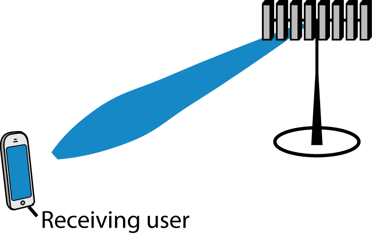
When an antenna array is used to focus a transmitted signal on a receiver, we call this beamforming (or precoding) and we usually illustrate it as shown to the right. This cartoonish illustration is only applicable when the antennas are gathered in a compact array and there is a line-of-sight channel to the receiver.
If we want to deploy very many antennas, as in Massive MIMO, it might be preferable to distribute the antennas over a larger area. One such deployment concept is called Cell-free Massive MIMO. The basic idea is to have many distributed antennas that are transmitting phase-coherently to the receiving user. In other words, the antennas’ signal components add constructively at the location of the user, just as when using a compact array for beamforming. It is therefore convenient to call it beamforming in both cases—algorithmically it is the same thing!
The question is: How can we illustrate the beamforming effect when using a distributed array?
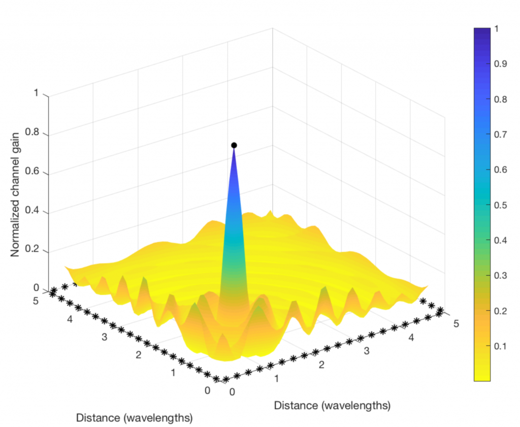
The figure below shows how to do it. I consider a toy example with 80 star-marked antennas deployed along the sides of a square and these antennas are transmitting sinusoids with equal power, but different phases. The phases are selected to make the 80 sine-components phase-aligned at one particular point in space (where the receiving user is supposed to be):
Clearly, the “beamforming” from a distributed array does not give rise to a concentrated signal beam, but the signal amplification is confined to a small spatial region (where the color is blue and the values on the vertical axis are close to one). This is where the signal components from all the antennas are coherently combined. There are minor fluctuations in channel gain at other places, but the general trend is that the components are non-coherently combined everywhere except at the receiving user. (Roughly the same will happen in a rich multipath channel, even if a compact array is used for transmission.)
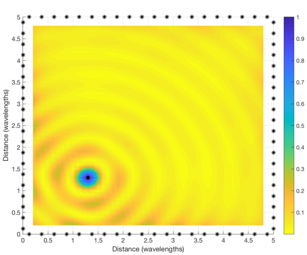
By looking at a two-dimensional version of the figure (see below), we can see that the coherent combination occurs in a circular region that is roughly half a wavelength in diameter. At the carrier frequencies used for cellular networks, this region will only be a few centimeters or millimeters wide. It is almost magical how this distributed array can amplify the signal at such a tiny spatial region! This spatial region is probably what the company Artemis is calling a personal cell (pCell) when marketing their distributed MIMO solution.
If you are into the details, you might wonder why I simulated a square region that is only a few wavelengths wide, and why the antenna spacing is only a quarter of a wavelength. This assumption was only made for illustrative purposes. If the physical antenna locations are fixed but we would reduce the wavelength, the size of the circular region will reduce and the ripples will be more frequent. Hence, we would need to compute the channel gain at many more spatial sample points to produce a smooth plot.
Reproduce the results: The code that was used to produce the plots can be downloaded from my GitHub.
Adaptive beamforming for wireless communications has a long history, with the modern research dating back to the 70s and 80s. There is even a paper from 1919 that describes the development of directive transatlantic communication practices that were developed during the First World War. Many of the beamforming methods that are considered today can be found already in the magazine paper Beamforming: A Versatile Approach to Spatial Filtering from 1988. Plenty of further work was carried out in the 90s and 00s, before the Massive MIMO paradigm.
I think it is fair to say that no fundamentally new beamforming methods have been developed in the Massive MIMO literature, but we have rather taken known methods and generalized them to take imperfect channel state information and other practical aspects into account. And then we have developed rigorous ways to quantify the achievable rates that these beamforming methods achieve and studied the asymptotic behaviors when having many antennas. Closed-form expressions are available in some special cases, while Monte Carlo simulations can be used to compute these expressions in other cases.
As beamforming has evolved from an analog phased-array concept, where angular beams are studied, to a digital concept where the beamforming is represented in multi-dimensional vector spaces, it easy to forget the basic properties of array processing. That is why we dedicated Section 7.4 in Massive MIMO Networks to describe how the physical beam width and spatial resolution depend on the array geometry.
In particular, I’ve observed a lot of confusion about the dimensionality of MIMO arrays, which are probably rooted in the confusion around the difference between an antenna (which is something connected to an RF chain) and a radiating element. I explained this in detail in a previous blog post and then exemplified it based on a recent press release. I have also recorded the following video to visually explain these basic properties:
A recent white paper from Ericsson is also providing a good description of these concepts, particularly focused on how an array with a given geometry can be implemented with different numbers of RF chains (i.e., different numbers of antennas) depending on the deployment scenario. While having as many antennas as radiating element is preferable from a performance perspective, but the Ericsson researchers are arguing that one can get away with fewer antennas in the vertical direction in deployments where it is anyway very hard to resolve users in the elevation dimension.
The tedious, time-consuming, and buggy nature of system-level simulations is exacerbated with massive MIMO. This post offers some relieve in the form of analytical expressions for downlink conjugate beamforming [1]. These expressions enable the testing and calibration of simulators—say to determine how many cells are needed to represent an infinitely large network with some desired accuracy. The trick that makes the analysis feasible is to let the shadowing grow strong, yet the ensuing expressions capture very well the behaviors with practical shadowings.
The setting is an infinitely large cellular network where each -antenna base station (BS) serves single-antenna users. The large-scale channel gains include pathloss with exponent and shadowing having log-scale standard deviation , with the gain between the th BS and the th user served by a BS of interest denoted by .With conjugate beamforming and receivers reliant on channel hardening, the signal-to-interference ratio (SIR) at such user is [2]
where is the gain from the serving BS and is the share of that BS’s power allocated to user . Two power allocations can be analyzed:
Uniform: .
SIR-equalizing [3]: , with the proportionality constant ensuring that . This makes . Moreover, as and grow large,
The analysis is conducted for , which makes it valid for arbitrary BS locations.
SIR
For notational compactness, let . Define as the solution to where is the lower incomplete gamma function. For , in particular, . Under a uniform power allocation, the CDF of is available in an explicit form involving the Gauss hypergeometric function (available in MATLAB and Mathematica):
where “” indicates asymptotic () equality, is such that the CDF is continuous, and
Alternatively, the CDF can be obtained by solving (e.g., with Mathematica) a single integral involving the Kummer function :
This latter solution can be modified for the SIR-equalizing power allocation as
Spectral Efficiency
The spectral efficiency of user is with CDF readily characterizable from the expressions given earlier. From , the sum spectral efficiency at the BS of interest can be found as Expressions for the averages and are further available in the form of single integrals.
With a uniform power allocation,
(1)
and . For the special case of , the Kummer function simplifies giving
(2)
With an equal-SIR power allocation
(3)
and .
Application to Relevant Networks
Let us now contrast the analytical expressions (computable instantaneously and exactly, and valid for arbitrary topologies, but asymptotic in the shadowing strength) with some Monte-Carlo simulations (lengthy, noisy, and bug-prone, but for precise shadowing strengths and topologies).
First, we simulate a 500-cell hexagonal lattice with , and . Figs. 1a-1b compare the simulations for – dB with the analysis. The behaviors with these typical outdoor values of are well represented by the analysis and, as it turns out, in rigidly homogeneous networks such as this one is where the gap is largest.
Figure 1: Analysis vs hexagonal network simulations with lognormal shadowing
For a more irregular deployment, let us next consider a network whose BSs are uniformly distributed. BSs (500 on average) are dropped around a central one of interest. For each network snapshot, users are then uniformly dropped until of them are served by the central BS. As before, , and . Figs. 2a-2b compare the simulations for dB with the analysis, and the agreement is now complete. The simulated average spectral efficiency with a uniform power allocation is b/s/Hz/user while (2) gives b/s/Hz/user.
Figure 2: Analysis vs Poisson network simulations with lognornmal shadowing.
The analysis presented in this post is not without limitations, chiefly the absence of noise and pilot contamination. However, as argued in [1], there is a broad operating range (– with very conservative premises) where these effects are rather minor, and the analysis is hence applicable.
Pilots are predefined reference signals that are transmitted to let the receiver estimate the channel. While many communication systems have pilot transmissions in both uplink and downlink, the canonical communication protocol in Massive MIMO only contains uplink pilots. In this blog post, I will explain when downlink pilots are needed and why we can omit them in Massive MIMO.
Consider the communication link between a single-antenna user and an -antenna base station (BS). The channel vector varies over time and frequency in a way that is often modeled as random fading. In each channel coherence blocks, the BS selects a precoding vector and uses it for downlink transmission. The precoding reduces the multiantenna vector channel to an effective single-antenna scalar channel
The receiving user does not need to know the full -dimensional vectors and . However, to decode the downlink data in a successful way, it needs to learn the complex scalar channel . The difficulty in learning depends strongly on the mechanism of precoding selection. Two examples are considered below.
Codebook-based precoding
In this case, the BS tries out a set of different precoding vectors from a codebook (e.g., a grid of beams, as shown to the right) by sending one downlink pilot signal through each one of them. The user measures for each one of them and feeds back the index of the one that maximizes the channel gain . The BS will then transmit data using that precoding vector. During the data transmission, can have any phase, but the user already knows the phase and can compensate for it in the decoding algorithm.
If multiple users are spatially multiplexed in the downlink, the BS might use another precoding vector than the one selected by the user. For example, regularized zero-forcing might be used to suppress interference. In that case, the magnitude of the channel changes, but the phase remains the same. If phase-shift keying (PSK) is used for communication, such that no information is encoded in the signal amplitude, no estimation of is needed for decoding (but it can help to reduce the error probability). If quadrature amplitude modulation (QAM) is used instead, the user needs to learn also to decode the data. The unknown magnitude can be estimated blindly based on the received signals. Hence, no further pilot transmission is needed.
Reciprocity-based precoding
In this case, the user transmits a pilot signal in the uplink, which enables the BS to directly estimate the entire channel vector . For the sake of argument, suppose this estimation is perfect and that maximum ratio transmission with is used for downlink data transmission. The effective channel gain will then be
which is a positive scalar. Hence, the user only needs to learn the magnitude of because the phase is always zero. Estimation of can be implemented without downlink pilots, either by relying on channel hardening or by blind estimation based on the received signals. The former only works well in Massive MIMO with very many antennas, while the latter can be done in any system (including codebook-based precoding).
Conclusion
We generally need to compensate for the channel’s phase-shift at some place in a wireless system. In codebook-based precoding, the compensation is done at the user-side, based on the received signals from the downlink pilots. This is the main approach in 4G systems, which is why downlink pilots are so commonly used. In contrast, when using reciprocity-based precoding, the phase-shifts are compensated for at the BS-side using the uplink pilots. In either case, explicit pilot signals are only needed in one direction: uplink or downlink. If the estimation is imperfect, there will be some remaining phase ambiguity, which can be estimated blindly since we know that it is small (i.e., of all possible phase-rotations that could have resulted in the received signal, the smallest one is most likely).
When we have access to TDD spectrum, we can choose between the two precoding methods mentioned above. The reciprocity-based approach is preferable in terms of less overhead signaling; one pilot per user instead of one per index in the codebook (the codebook size needs to grow with the number of antennas), and no feedback is needed. That is why this approach is taken in the canonical form of Massive MIMO.
The user terminals in reciprocity-based Massive MIMO transmit two types of uplink signals: data and pilots (a.k.a. reference signals). A terminal can potentially transmit these signals using different power levels. In the book Fundamentals of Massive MIMO, the pilots are always sent with maximum power, while the data is sent with a user-specific power level that is optimized to deliver a certain per-user performance. In the book Massive MIMO networks, the uplink power levels are also optimized, but under another assumption: each user must assign the same power to pilots and data.
Moreover, there is a series of research papers (e.g., Ref1, Ref2, Ref3) that treat the pilot and data powers as two separate optimization variables that can be optimized with respect to some performance metric, under a constraint on the total energy budget per transmission/coherence block. This gives the flexibility to “move” power from data to pilots for users at the cell edge, to improve the channel state information that the base station acquires and thereby the array gain that it obtains when decoding the data signals received over the antennas.
In some cases, it is theoretically preferable to assign, for example, 20 dB higher power to pilots than to data. But does that make practical sense, bearing in mind that non-linear amplifiers are used and the peak-to-average-power ratio (PAPR) is then a concern? The answer depends on how the pilots and data are allocated over the time-frequency grid. In OFDM systems, which have an inherently high PAPR, it is discouraged to have large power differences between OFDM symbols (i.e., consecutive symbols in the time domain) since this will further increase the PAPR. However, it is perfectly fine to assign the power in an unequal manner over the subcarriers.
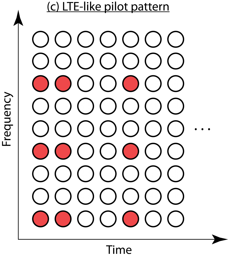
In the OFDM literature, there are two elementary ways to allocate pilots: block and comb type arrangements. These are illustrated in the figure below and some early references on the topic are Ref4, Ref5, Ref6.
(a): In the block type arrangement, at a given OFDM symbol time, all subcarriers either contain pilots or data. It is then preferable for a user terminal to use the same transmit power for pilots and data, to not get a prohibitively high PAPR. This is consistent with the assumptions made in the book Massive MIMO networks.
(b): In the comb type arrangement, some subcarriers always contain pilots and other subcarriers always contain data. It is then possible to assign different power to pilots and data at a user terminal. The power can be moved from pilot subcarriers to data subcarriers or vice versa, without a major impact on the PAPR. This approach enables the type of unequal pilot and data power allocations considered in Fundamentals of Massive MIMO or research papers that optimize the pilot and data powers under a total energy budget per coherence block.
The downlink in LTE uses a variation of the two elementary pilot arrangements, as illustrated in (c). It is easiest described as a comb type arrangement where some pilots are omitted and replaced with data. The number of omitted pilots depend on how many antenna ports are used; the more antennas, the more similar the pilot arrangement becomes to the comb type. Hence, unequal pilot and power allocation is possible in LTE but maybe not as easy to implement as described above. 5G has a more flexible frame structure but supports the same arrangements as LTE.
In summary, uplink pilots and data can be transmitted at different power levels, and this flexibility can be utilized to improve the performance in Massive MIMO. It does, however, require that the pilots are arranged in practically suitable ways, such as the comb type arrangement.
Drones could shape the future of technology, especially if provided with reliable command and control (C&C) channels for safe and autonomous flying, and high-throughput links for multi-purpose live video streaming. Some months ago, Prabhu Chandhar’s guest post discussed the advantages of using massive MIMO to serve drone – or unmanned aerial vehicle (UAV) – users. More recently, our Paper 1 and Paper 2 have quantified such advantages under the realistic network conditions specified by the 3GPP. While demonstrating that massive MIMO is instrumental in enabling support for UAV users, our works also show that merely upgrading existing base stations (BS) with massive MIMO might not be enough to provide a reliable service at all UAV flying heights. Indeed, hardware solutions need to be complemented with signal processing enhancements through all communications phases, namely, 1) UAV cell selection and association, 2) downlink BS-to-UAV transmissions, and 3) uplink UAV-to-BS transmissions. These are outlined below.
1. UAV cell selection and association
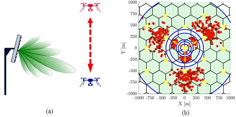
As depicted in Figure 1(a), most existing cellular BSs create a fixed beampattern towards the ground. Thanks to this, ground users tend to perceive a strong signal strength from nearby BSs, which they use for connecting to the network. Instead, aerial users such as the red drone in Figure 1(a) only receive weak sidelobe-generated signals from a nearby BS when flying above it. This results in a deployment planning issue as illustrated in Figure 1(b), where due to the radiation of a strong sidelobe, the tri-sector BSs located in the origin can be the preferred server for far-flung UAVs (red spots). Consequently, these UAVs might experience strong interference, since they perceive signals from a multiplicity of BSs with similar power.
Figure 1. (a) Illustration of a downtilted cellular BS and its beampattern: low (blue) UAV receives strong main lobe signals, whereas high (red) drone only receives weak sidelobe-generated signals. (b) 150-meter-high UAVs (red dots) associated with a three-cell BS site located at the origin and pointing at 30°, 150°, and 270°. The three BSs of each cellular site (orange squares) generate ground cells represented by hexagons.
On the other hand, thanks to their capability of beamforming the synchronization signals used for user association, massive MIMO systems ensure that aerial users generally connect to a nearby BS. This optimized association enhances the robustness of the mobility procedures, as well as the downlink and uplink data phases.
2. Downlink BS-to-UAV transmissions
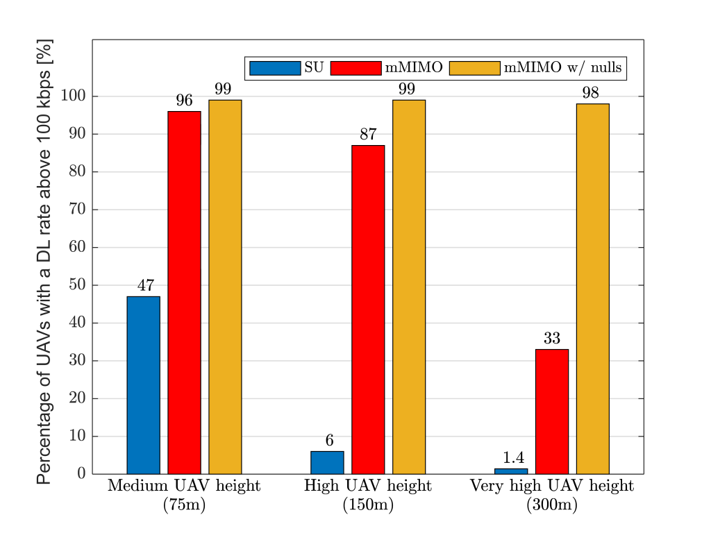
During the downlink data phase, UAV users are very sensitive to the strong inter-cell interference generated from a plurality of BSs, which are likely to be in line-of-sight. This may result in performance degradation, preventing UAVs from receiving critical C&C information, which has an approximate rate requirement of 60-100 kbps. Indeed, Figure 2 shows how conventional cellular networks (‘SU’) can only guarantee 100 kbps to a mere 6% of the UAVs flying at 150 meters. A conventional massive MIMO system (‘mMIMO’) enhances the data rates, albeit only 33% of the UAVs reach 100 kbps when they fly at 300 meters. This is due to a well-known effect: pilot contamination. Such an effect is particularly severe in scenarios with UAV users, since they can create strong uplink interference to many line-of-sight BSs simultaneously. In contrast, the pilot contamination decays much faster with distance for ground UEs.
In a nutshell, Figure 2 tells us that complementing conventional massive MIMO with explicit inter-cell interference suppression (‘mMIMO w/ nulls’) is essential when supporting high UAVs. In a ‘mMIMO w/ nulls’ system, BSs incorporate additional signal processing features that enable them to perform a twofold task. First, leveraging channel directionality, BSs can spatially separate non-orthogonal pilots transmitted by different UAVs. Second, by dedicating a certain number of spatial degrees of freedom to place radiation nulls, BSs can mitigate interference on the directions corresponding to users in other cells that are most vulnerable to the BS’s interference. Indeed, these additional capabilities dramatically increase the percentage of UAVs that meet the 100 kbps requirement when these are flying at 300 m, from 33% (‘mMIMO’) to a whopping 98% (‘mMIMO w/ nulls’).
Figure 2. Percentage of UAVs with a downlink C&C rate above 100 kbps for three representative UAV heights. ‘SU’ denotes a conventional cellular network with a single antenna port, ‘mMIMO’ represents a system with 8×8 dual-polarized antenna arrays and 128 antenna ports, and ‘mMIMO w/ nulls’ complements the latter with additional space-domain inter-cell interference suppression techniques.
3. Uplink UAV-to-BS transmissions
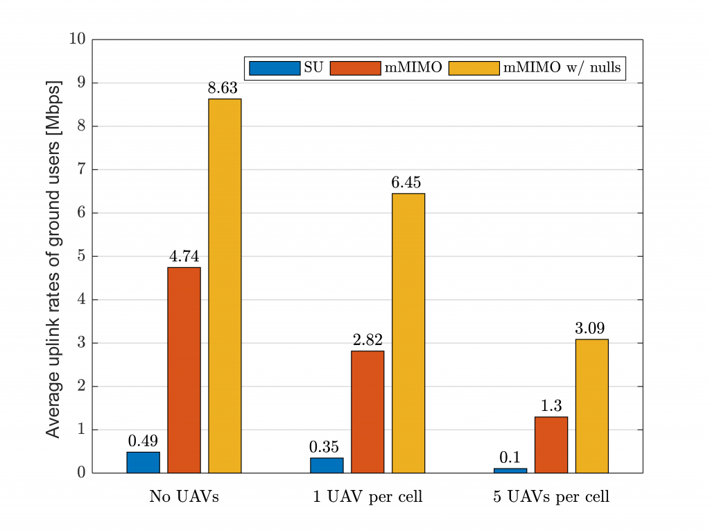
Unlike the downlink, where UAVs should be protected to prevent a significant performance degradation, it is the ground users who we should care about in the uplink. This is because line-of-sight UAVs can generate strong interference towards many BSs, therefore overwhelming the weaker signals transmitted by non-line-of-sight ground users. The consequences of such a phenomenon are illustrated in Figure 3, where the uplink rates of ground users plummet as the number of UAVs increases.
Again, ‘mMIMO w/nulls’ – incorporating additional space-domain inter-cell interference suppression capabilities – can solve the above issue and guarantee a better performance for legacy ground users.
Figure 3. Average uplink rates of ground users when the number of UAVs per cell grows. ‘SU’ denotes a conventional cellular network with a single antenna port, ‘mMIMO’ represents a system with 8×8 antenna dual-polarized antenna arrays and 128 antenna ports, and ‘mMIMO w/ nulls’ complements the latter with additional space-domain inter-cell interference suppression techniques.
Overall, the efforts towards realizing aerial wireless networks are just commencing, and massive MIMO will likely play a key role. In the exciting era of fly-and-connect, we must revisit our understanding of cellular networks and develop novel architectures and techniques, catering not only for roads and buildings, but also for the sky.


 -antenna base station (BS) serves
  single-antenna users. The large-scale channel gains include pathloss with exponent
  and shadowing having log-scale standard deviation
  , with the gain between the
  th BS and the
  th user served by a BS of interest denoted by
  .
.
 is the gain from the serving BS and
  is the share of that BS’s power allocated to user
  .
. , with the proportionality constant ensuring that
  . This makes
  . Moreover, as
 , which makes it valid for arbitrary BS locations.
 . Define
  as the solution to
  where
where  is the lower incomplete gamma function. For
  , in particular,
  . Under a uniform power allocation, the CDF of
  is available in an explicit form involving the Gauss hypergeometric function
  (available in MATLAB and Mathematica):
 ” indicates asymptotic (
 ) equality,
  is such that the CDF is continuous, and
 :
:

 with CDF
  readily characterizable from the expressions given earlier. From
  , the sum spectral efficiency at the BS of interest can be found as
  Expressions for the averages
 ![\bar{C} = \mathbb{E} \big[ C_k \big]](http://ma-mimo.ellintech.se/wp-content/ql-cache/quicklatex.com-a887caab28778e8d91a237bcc86a9f3e_l3.png "Rendered by QuickLaTeX.com") and
and ![\bar{C}_{\scriptscriptstyle \Sigma} = \mathbb{E} \! \left[ C_{\scriptscriptstyle \Sigma} \right]](http://ma-mimo.ellintech.se/wp-content/ql-cache/quicklatex.com-865de5351a43ee6f0405ddb531ed84ee_l3.png "Rendered by QuickLaTeX.com") are further available in the form of single integrals.
are further available in the form of single integrals.
 . For the special case of

 ,
,  and
and  –
– dB with the analysis. The behaviors with these typical outdoor values of
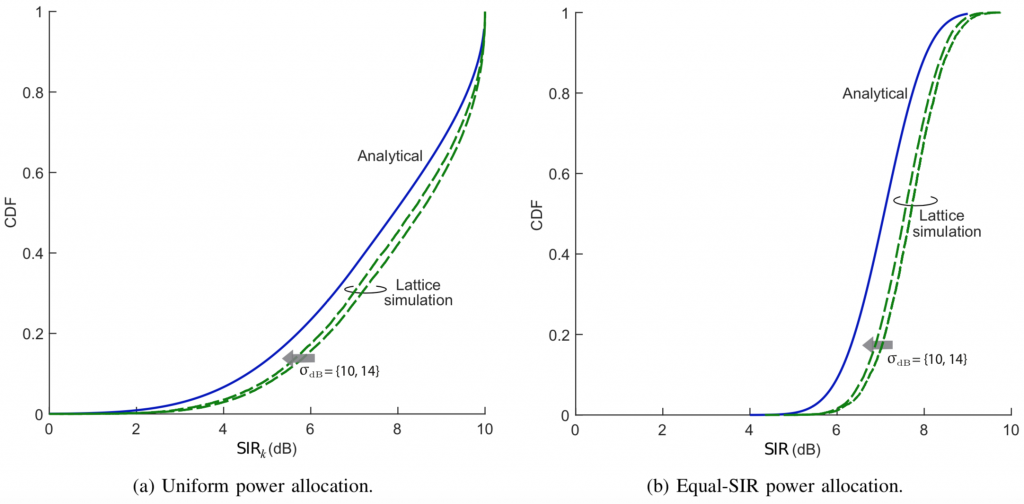
 and
and  . Figs. 2a-2b compare the simulations for
  dB with the analysis, and the agreement is now complete. The simulated average spectral efficiency with a uniform power allocation is
  b/s/Hz/user while (2) gives
  b/s/Hz/user.
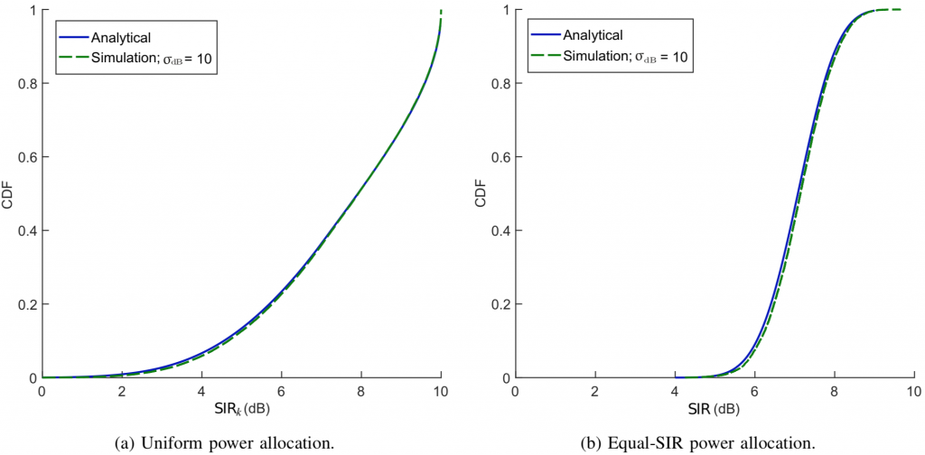
 –
– with very conservative premises) where these effects are rather minor, and the analysis is hence applicable.
 -antenna base station (BS). The channel vector
  varies over time and frequency in a way that is often modeled as random fading. In each channel coherence blocks, the BS selects a precoding vector
  and uses it for downlink transmission. The precoding reduces the multiantenna vector channel to an effective single-antenna scalar channel
 and
and  . However, to decode the downlink data in a successful way, it needs to learn the complex scalar channel
  . The difficulty in learning
 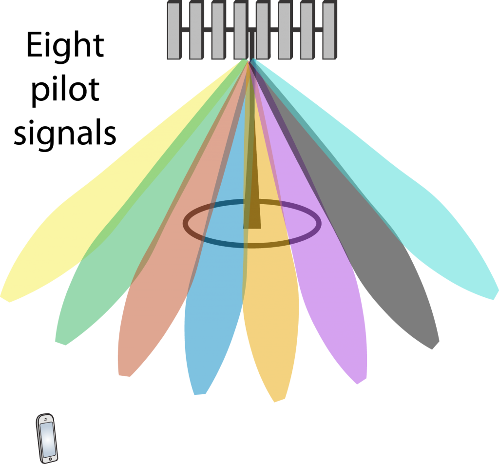 In this case, the BS tries out a set of different precoding vectors from a codebook (e.g., a grid of beams, as shown to the right) by sending one downlink pilot signal through each one of them. The user measures
  . The BS will then transmit data using that precoding vector. During the data transmission,
  can have any phase, but the user already knows the phase and can compensate for it in the decoding algorithm.
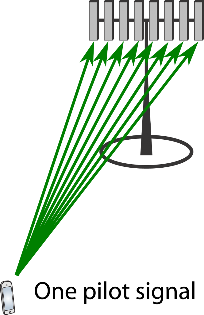 In this case, the user transmits a pilot signal in the uplink, which enables the BS to directly estimate the entire channel vector
  is used for downlink data transmission. The effective channel gain will then be