
When researchers study the basic properties of multi-antenna technologies, it is a common practice to model the channels using independent and identically distributed (i.i.d.) Rayleigh fading. This practice goes back many decades and is convenient since: 1) every antenna observes an independent realization of the channel; 2) each antenna is statistically equally good, so the ordering doesn’t matter; 3) the channel coefficients are complex Gaussian distributed, which leads to convenient mathematics.
The i.i.d. Rayleigh fading model has become the baseline that is considered unless the research is explicitly focused on a different model. When using the model to study spatial diversity, the diversity gain becomes proportional to the number of antennas. When characterizing the ergodic capacity of Massive MIMO, one can derive simple closed-form bounds where the SINR is proportional to the number of antennas. Both results are correct, but their generality is limited by the generality of the underlying fading model. Hence, it is important to know under what conditions i.i.d. Rayleigh fading can be observed.
When i.i.d. fading might occur
In isotropic scattering environments, where the multi-path components are uniformly distributed over all directions (in three dimensions), the fading realizations observed at two points have a correlation determined by the distance d between them. More precisely, the cross-correlation is sinc(2d/λ), where λ is the wavelength. The sinc function is zero when the argument is a non-zero integer, thus the fading realizations at two different points are uncorrelated if and only if they are separated by an integer multiple of λ/2. For example, d = λ/2, λ, 3λ/2, etc. Since the channel coefficients are Gaussian distributed in isotropic fading, uncorrelated fading results in independent fading.
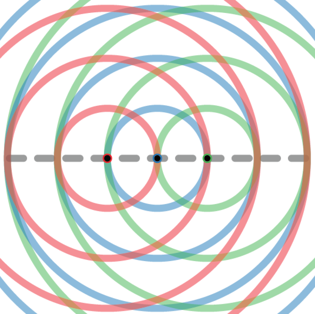
The figure above illustrates a setup where 3 antennas are deployed on the dashed line with a separation of λ/2. The red circles around the “red antenna” show at which locations one can observe fading realizations that are independent of the observation made at the red antenna. The circles have radius λ/2, λ, 3λ/2, etc. The blue and green circles have the same meanings for the blue and green antennas, respectively. Since all the antennas are deployed on the circles of the other antennas, they will observe mutually uncorrelated (independent) fading. This will give rise to i.i.d. Rayleigh fading.
Suppose we want to deploy a fourth antenna. To retain an i.i.d. fading distribution, we must put it at a point where a red, a blue, and a green circle intersect. As indicated by the figure, such points are only be found along the dashed line. Hence, a uniform linear array (ULA) with λ/2-separation between the adjacent antennas will observe i.i.d. fading if deployed in an isotropic scattering environment.
When i.i.d. fading cannot occur
Apart from the ULA example, there is essentially no other case where i.i.d. fading can occur. This is important since two-dimensional planar arrays are becoming standard, for example, when deploying Massive MIMO in cellular networks. Even if we allow ourselves to deviate from the isotropic scattering assumption, any physically accurate stochastic channel model for planar arrays exhibits correlation. This is proved in the paper “Spatially-Stationary Model for Holographic MIMO Small-Scale Fading“.
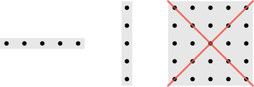
The horizontal and vertical ULAs in the figure above can observe i.i.d. fading, while the planar array cannot; even if the horizontal and vertical antenna spacing is λ/2, the spacings along the diagonals are different.
Looking further into the future, two new array concepts are currently receiving attention from the research community:
- Large intelligent surfaces (LIS);
- Reconfigurable intelligent surfaces (RIS).
LIS are large active arrays, while RIS are large passive arrays with elements that scatter incident signals in a semi-controllable fashion. In both cases, the word “surface” signifies that at a planar array, or even a three-dimensional array, is considered. Hence, these arrays can never observe i.i.d. fading—it is physically impossible. Moreover, a key characteristic of LIS and RIS is that the element spacing is smaller than λ/2 (to approximate a continuously controllable surface), which is yet another reason for obtaining spatial channel correlation. It is therefore worrying that several early papers on these topics are making use of the i.i.d. fading model: the analysis might be beautiful but the results are insignificant since they cannot be observed in practice.
The way forward
Even if we have reached the end of the road for the i.i.d. Rayleigh fading model, we don’t have to wander into the darkness. We just need to switch to utilizing the more general spatially correlated Rayleigh fading model. There is already a rich literature on how to design communication systems for such channels. My book “Massive MIMO networks” is one possible starting point, but not the only one.
To make the transition to physically accurate models easier, I have co-authored the paper “Rayleigh Fading Modeling and Channel Hardening for Reconfigurable Intelligent Surfaces“, which derives a spatial correlation model for LIS and RIS in isotropic scattering environments. It can take the role as the new baseline channel model that is used when no other specific channel model is studied. We also elaborate on why the classical “Kronecker approximation” of spatial correlation matrices is inaccurate; for example, it results in i.i.d. fading also for planar arrays.
There are exactly 3 ways to tile a 2D plane with regular polygons:
equilateral triangle, square, regular hexagon. A 2D array can be arranged with equilateral triangles, with edge length = λ/2.
Yes, that is correct. But none of them will lead to i.i.d. fading (except for the case of a single equilateral triangle), since one cannot guarantee that all elements are separated by a distance of integer*λ/2.
But is it that really important to get perfect zero correlation? Beyond lambda/2, cross correlation between observed channels is below 10% (assuming Rayleigh channel) and if we have some space to keep the antennas even more separated, that value is even lower. Considering that real environments are not isotropic, I feel that this might not be such a serious issue ¿?¿?
When analyzing just a single communication link, neglecting the correlation might not lead to any major performance differences. However, I think a research methodology where i.i.d. fading is assumed is somewhat deceiving since the reader will get the impression that the analysis is rigorous since the approximations are hidden in the assumptions. As you are saying, real environments are not isotropic so there will always be correlation for that reason. So far, people who are anyway using i.i.d. fading models could motivate this with the use of ULAs in isotropic fading, but now when LIS/RIS research focus on two-dimensional arrays, that argument cannot be used anymore. That is why I think that we should stop using i.i.d. fading models in that literature.
When serving multiple users, it is the spatial correlation properties that determine how well the users can be separated. We will get rank-deficient correlation matrices and this will affect how to estimate channels, how well one can separate users, how many users can be multiplexed at the same time, and how properties such as channel hardening behaves. This is what we write about in the paper https://arxiv.org/pdf/2009.04723.pdf
Sorry Emil, I can’t follow your reasoning. If my understanding is correct, in your document you say that placing antennae as in ULA at half-wavelength distance, we would have independent Rayleigh fading at the receivers. However, the correlation among the received signals depends on the distance *of the receiver* from each of the transmitting antenna, and these distances are usually not integer multiples of half-wavelength (except when the receiver lies on the same plan of the transmitting antennae). Isn’t that correct? According to my understanding, perfect independence is (theoretically) rather unlikely, though the correlation drops very quickly with the distance from the transmitter (particularly so for short wavelengths), so that engineers can safely assume independent fadings in most practical cases.
My reasoning is based on an isotropic scattering environment, where there are infinitely many multipath components, each with an intensity that is drawn from the same distribution. In such a stochastic environment, there is no notion of distances and the spatial correlation is a sinc-function (this is the classical 3D Clarke’s model).
I’m not sure what kind of fading environment that you have in mind. If there is only one direct path, then there won’t be any fading and, thus, the channel coefficients will be perfectly correlated. If you consider a one-ring-like scattering model, with multi-path components arriving from within an angular interval, there will be fading and spatial correlation. It is the width of the angular interval that determines the spatial correlation, so if you increase the propagation distance while keeping the “ring” fixed in size, you will get more spatial correlation since the angular interval shrinks.
With a 2D array, engineers cannot safely assume independent fading since it cannot ever be observed. This is the main point. Even in the most rich scattering situations, 21% of the eigenvalues in the correlation matrix will be approximately zero, while an i.i.d. model will get 0% eigenvalues that are like that. The implications of this are discuss in https://arxiv.org/pdf/2009.04723.pdf and the result itself is proved in this paper: https://arxiv.org/abs/1911.04853
Dear Dr. Emil,
In your paper, “Rayleigh Fading Modeling and Channel Hardening for Reconfigurable Intelligent Surfaces“, you consider a single-antenna transmitter communicating with a single-antenna receiver in an isotropic scattering environment, while being aided by an RIS equipped with N reconfigurable elements.
However, I’d like to understand and have a grasp on the model for a system where the single-antenna transmitter is replaced by a M antenna one. In this case, how could we model the correlation since the M and the N antenna arrays would have different correlations matrices?
Thanks and Kind Regards,
Felipe
There will then be correlation between the channels that can be described by something that was previously called the Weichselberger model. Here is a recent derivation of it: https://arxiv.org/pdf/2012.07389.pdf
You can focus on Section IV