
The channel between a single-antenna user and an  -antenna base station can be represented by an -dimensional channel vector. The canonical channel model in the Massive MIMO literature is independent and identically distributed (i.i.d.) Rayleigh fading, in which the vector is a circularly symmetric complex Gaussian random variable with a scaled identity matrix as correlation/covariance matrix:
  , where
  is the variance.
With i.i.d. Rayleigh fading, the channel gain  has an Erlang
 -distribution (this is a scaled
  distribution) and the channel direction
  is uniformly distributed over the unit sphere in
  . The channel gain and the channel direction are also independent random variables, which is why this is a spatially uncorrelated channel model.
One of the key benefits of i.i.d. Rayleigh fading is that one can compute closed-form rate expressions, at least when using maximum ratio or zero-forcing processing; see Fundamentals of Massive MIMO for details. These expressions have an intuitive interpretation, but should be treated with care because practical channels are not spatially uncorrelated. Firstly, due to the propagation environment, the channel vector is more probable to point in some directions than in others. Secondly, the antennas have spatially dependent antenna patterns. Both factors contribute to the fact that spatial channel correlation always appears in practice.
One of the basic properties of spatial channel correlation is that the base station array receives different average signal power from different spatial directions. This is illustrated in Figure 1 below for a uniform linear array with 100 antennas, where the angle of arrival is measured from the boresight of the array.
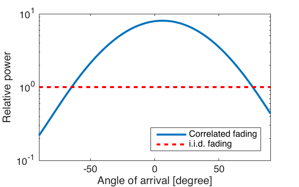
As seen from Figure 1, with i.i.d. Rayleigh fading the average received power is equally large from all directions, while with spatially correlated fading it varies depending on in which direction the base station applies its receive beamforming. Note that this is a numerical example that was generated by letting the signal come from four scattering clusters located in different angular directions. Channel measurements from Lund University (see Figure 4 in this paper) show how the spatial correlation behaves in practical scenarios.
Correlated Rayleigh fading is a tractable way to model a spatially correlation channel vector:  , where the covariance matrix
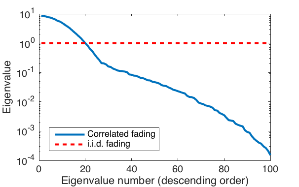
  is also the correlation matrix. It is only when is a scaled identity matrix that we have spatially uncorrelated fading. The eigenvalue distribution determines how strongly spatially correlated the channel is. If all eigenvalues are identical, then is a scaled identity matrix and there is no spatial correlation. If there are a few strong eigenvalues that contain most of the power, then there is very strong spatial correlation and the channel vector is very likely to be (approximately) spanned by the corresponding eigenvectors. This is illustrated in Figure 2 below, for the same scenario as in the previous figure. In the considered correlated fading case, there are 20 eigenvalues that are larger than in the i.i.d. fading case. These eigenvalues contain 94% of the power, while the next 20 eigenvalues contain 5% and the smallest 60 eigenvalues only contain 1%. Hence, most of the power is concentrated to a subspace of dimension
  . The fraction of strong eigenvalues is related to the fraction of the angular interval from which strong signals are received. This relation can be made explicit in special cases.
One example of spatially correlated fading is when the correlation matrix has equal diagonal elements and non-zero off-diagonal elements, which describe the correlation between the channel coefficients of different antennas. This is a reasonable model when deploying a compact base station array in tower. Another example is a diagonal correlation matrix with different diagonal elements. This is a reasonable model when deploying distributed antennas, as in the case of cell-free Massive MIMO.
Finally, a more general channel model is correlated Rician fading:  , where the mean value
  represents the deterministic line-of-sight channel and the covariance matrix determines the properties of the fading. The correlation matrix
  can still be used to determine the spatial correlation of the received signal power. However, from a system performance perspective, the fraction
  between the power of the line-of-sight path and the scattered paths can have a large impact on the performance as well. A nearly deterministic channel with a large
  -factor provide more reliable communication, in particular since under correlated fading it is only the large eigenvalues of that contributes to the channel hardening (which otherwise provides reliability in Massive MIMO).
How to make reconfigurable MIMO antenna arrays at 5G frequencies using phase shifters for wireless devices?
Massive MIMO should be built with fully digital transceivers. Analog beamforming with phase shifters will only work satisfactory in special cases: single user communication with phase-calibrated arrays, line of sight propagation and a relatively small bandwidth.
How does spatial correlation impact the channel capacity (data rate). Is there any tradeoff between spatial channel correlation and spectral efficiency? I would like write a paper on spatial channel correlation.
It depends on how the users are distributed. Users with similar spatial channel correlation will cause more interference to each other, while users with very different spatial channel correlation cause less interference to each other. On the average, it appears that spatial channel correlation improves the spectral efficiency.
This is discussed in depth in my new book, so I suggest that you read it before conducting research on the topic:
Emil Björnson, Jakob Hoydis and Luca Sanguinetti (2017), “Massive MIMO Networks: Spectral, Energy, and Hardware Efficiency”, Foundations and Trends® in Signal Processing: Vol. 11, No. 3-4, pp 154–655. DOI: 10.1561/2000000093.
Dear Professor,
I have a question.
Question: Can we use “AMP Algorithm” in “Correlated Rayleigh Fading Model” for Activity Detection of active user?
Actually I am working on massive connectivity but I have seen many researchers follow i.i.d fading channel instead of Correlated fading channel.
Yes, I think so.
It is often more analytically tractable to deal with i.i.d. fading channels, which is why many research advances are first made for i.i.d. channels and then generalized to correlated fading.
Dear Emil,
I’m interested to know more about what you said:
“On the average, it appears that spatial channel correlation improves the spectral efficiency.”
Can you please suggest the chapter of your book and any other paper, where explains this a little bit…?
Check out Figure 4.8 and the associated text in my book Massive MIMO Networks, https://massivemimobook.com
Sections 3 and 4 explain these things in more detail.
Thanks
How to generate interchannel correlation matrix in Matlab? I’m considering the scenario of multi-user MIMO, where users are close to each other.
It is commonly assumed that the channel realizations of different users are statistically independent in the multi-user MIMO literature, even when the users are close to each other. With this assumption, the inter channel correlation matrix is zero.
But if you want to generate more realistic channels that have some correlation, you can use the following Matlab implementation of 3GPP channel models:
http://quadriga-channel-model.de
Is spatial correlation measurable? Can we quantity it?
Yes, several different methods to estimate the spatial correlation matrices are described in this paper: https://arxiv.org/pdf/1904.03406
Sir, is spatial correlation measurable in any unit?
There is unfortunately not a simple way to measure spatial correlation. One way to measure it is via the eigenvalue spread of the spatial correlation matrices, as illustrated in Figure 2.6 of my book “Massive MIMO networks” (http://massivemimobook.com). A strongly correlated channel has a few large eigenvalues and many small eigenvalues. But if you compare the three curves in Figure 2.6, it is not easy to say that one is more correlated than the other.
If you consider a particular type of channel model, the spatial correlation might be determined by a parameter. In particular, the “angular spread” is a common measure for spatial correlation in physical propagation models (such as the one used in Figure 2.6). A smaller angular spread corresponds to stronger spatial correlation.
Dear Professor,
I have a question about the spatial correlation matrix.
As you also wrote in one of your paper that I’m studying, the eigenstructure of the correlation matrix (R) determines the spatial correlation properties of the channel (H).
Lets suppose we have Nt transmit antennas (1 BS only) and K single-antenna users (it could be also one point-to-point MIMO, system with only 1 user with Nr antennas… yes, they are not actually the same situation, but I want to focus on a different point).
In this situation we have a K-by-Nt channel matrix H.
Now, my very simple question is: what’s the spatial correlation matrix R?
Because from “MIMO Wireless Networks. Channels, Techniques and Standards for Multi-Antenna, Multi-User and Multi-Cell Systems (C. Oestges), section 2.3”, R is given as
R = E{vec(H)’ * vec(H)},
which is a K*Nt-by-K*Nt matrix. (E{*} is the expectation operator).
Then it talks about also the transmit correlation matrix (Rt) and the receive correlation matrix (Rr). In any simulation I’m running, I got just one eigenvalue of R (all the others are zero), and n=rank(H) eigenvalues of Rt/Rr. Moreover, the eigenvalue of R is always the sum of all eigenvalues of Rt/Rr.
I have not clear the role of R with respect to Rt or Rr.
Thank you very much, and sorry for the long comment.
Leo
Section 2.3 in the book by Clerckx and Oestges considers point-to-point MIMO channels. In this case, you can compute covariance matrix as R = E{ vec(H)’ * vec(H)}. If the channel is modeled as H = Rr^(1/2) * Hiid * Rt^(1/2), where Hiid has i.i.d. elements, then R = Rt^T (kronecker product) Rr.
When there are multiple users, you should compute a different matrix R for every user. One should not mix them together into a single covariance matrix – that will only cause confusion and complicate things.
Hi Emil, just reading through this post and comments to it. Thanks for putting it together.
In the comment above you wrote that in measuring spatial correlation one should not mix correlation matrices of different users. But how would you quantify the level of correlation between multiple users otherwise? Is there a good measure for that?
I notice occasionally that papers that study multi-user MIMO systems are using correlated channel models from the single-user (point-to-point) MIMO literature. This is what my previous response was referring to. The popular Kronecker channel model shouldn’t be used to study multi-user MIMO because 1) The user channels are normally not correlated; 2) The correlation matrix from the BS to each of the users will normally be different.
So to answer your question, there is no need to quantify the _statistical_ correlation between the user channels, because their fading realizations are normally assumed to be independent.
If one is not talking about statistical correlation but a broader sense of correlation, then one can come to other conclusions. Two users with independent channel realizations but similar spatial correlation matrices will interfere more with each other than two users with very different correlation matrices. One possible metric of this is the correlation matrix distance described in the paper “Correlation matrix distance, a meaningful measure for evaluation of non-stationary MIMO channels” (https://publik.tuwien.ac.at/files/pub-et_10119.pdf).
For two matrices A and B, it is 1-tr(A*B)/norm(A)/norm(B), using the Frobenius norms.
Dear Professor,
I have read about the Local Scattering Spatial Correlation Model in your book and I would like to ask what is your opinion about Kronecker, Weichselberger, and exponential channel model? I think that they are not the most suitable models to represent real conditions but are they good enough to estimate the BER performance of a linear detector such as Zero-Forcing?
The exponential correlation model is an actual method to generate spatial correlation matrices. It is analytically convenient since one can vary one parameter to determine the level of correlation. But it is not especially physically accurate.
Kronecker and Weichselberger models are not used to generate spatial correlation matrices, but to impose a special structure on single-user point-to-point MIMO channels. They are describing how the channels observed at the transmit arrays and receiver array are correlated. The Weichselberger model is more general than the Kronecker model. In my book and many Massive MIMO papers, single-antenna users are assumed and then Kronecker and Weichselberger model doesn’t really exist – the structure that they impose only make a difference when there are multiple antennas at the users as well.
Thanks for your answer.
I am going to use the Local Scattering Spatial Correlation Model from your book for my simulations because I deal with multi-user MIMO systems. I thought that the Kronecker model could also impose a special structure on multi-user point-to-point MIMO channels. There are many papers which are using the Kronecker model and they refer to their system as a massive MIMO system. So I was confused because I have on my mind that a massive MIMO system is a multi-user MIMO.
One more thing I would like to ask. Could a single-user MIMO system with 128 receiving antennas (BS) and 16 transmitting antennas have a practical use or for this number of antennas only multi-user MIMO systems are examined?
I’m sure you can find confusing statements in published papers. Not everything that is said papers is correct, not even in my papers… 🙂
Yes, particularly, in mmWave bands where 16 antennas can be easily squeezed into a user device (in fact, it might be needed to get a decent SNR). A rule-of-thumb is that each antenna is lambda/2 x lambda/2, thus the total area of 16 antennas is 4*lambda^2. If lambda = 1 cm (30 GHz), then the array will have an area of 4 cm^2, for example, configured as a square of size of 2 cm x 2 cm. That is not much!
1) by which parameter level or amount of correlation can be controlled?
2) how to measure level or amount of correlation?
3) firstRow(column,n) = exp(1i*2*pi*antennaSpacing*sin(thetaN)*distance)*exp(-((ASD^2)/2) * ( 2*pi*antennaSpacing*cos(thetaN)*distance )^2); is this exponential correlation model based covariance matrix first row equation?
above three questions are in reference to covariance matrix.
Spatial correlation can be measured in terms of the eigenvalue spread of the correlation matrix, but there is no simple way to say that one channel is more correlated than another one.
Some theoretical models have a parameter that controls the spatial correlation. In the exponential model, one increases the parameter’s absolute value to increase the correlation. In the local scattering model, one reduces the angular spread to increase the correlation.
I think that the code that you mention is for the (approximate) local scattering model, described in Chapter 2 of my book Massive MIMO networks. That chapter provides an in-depth description of these things.
Dear Emil,
You mentioned that “On the average, it appears that spatial channel correlation improves the spectral efficiency.”
In one of your paper titled “Performance analysis of cell-free massive MIMO over spatially correlated fading channels” (https://ieeexplore.ieee.org/document/8762051) you showed that spatial correlation degrades the spectral efficiency, here you have taken randomly distributed setups.
In another paper titled “Massive MIMO with Spatially Correlated Rician Fading Channels”, the code you have provided for this on Github. Using this code I have checked for ASD 10, 30 degree and plotted the SE. What I found is that spectral efficiency (with ASD 10) is greater than the spectral efficiency (with ASD 30) for both Rician, Rayleigh channels, and SE with the uncorrelated case is lower than than ASD 10, 30.
In both papers, you have considered randomly distributed channels.
None of the published papers has shown that spatial correlation improves SE.
In the first paper (cell-free network), the SE degrades with increasing spatial correlation even though the users are randomly distributed. I would like to ask that how in cell-free systems the SE degrades with increasing spatial correlation, but not in the multi-cell paper. (second paper). Can you please explain my doubt, I have read your book on massive MIMO there you mentioned that “as a UE moves around in the network the probability of achieving a particular SE is consistently higher under spatial correlation”.
The quoted statement is based on my experience from the numerical experiments that I carried out while writing the book “Massive MIMO networks”. For example, Figure 4.7 in the book shows how the SE is higher when the ASD is low compared to when it is high. Note that low ASD represents a high spatial correlation. Hence, if you observed from my code that ASD 10 gives a higher SE than ASD 30, then this is in line with my hypothesis that higher spatial correlation leads to higher SE.
The situation might be different in cell-free systems. I haven’t studied the impact of spatial correlation in detail in such systems, but I have seen some inconsistent results of the kind that you refer to. If I have to guess, I think the problem has to do with channel hardening, or the lack of it. Higher spatial correlation leads to less channel hardening. That is not a big deal in Massive MIMO with 100 antennas, but it might be a big deal in cell-free Massive MIMO if you are using capacity bounds that are tighter the more channel hardening there is. Maybe that explain the results from “Performance analysis of cell-free massive MIMO over spatially correlated fading channels”.
Hi there,
I know that if the LOS is clear and the multipath is sparse, one lambda distance unlikely provides enough spatial diversity (in other words, two antenna’s channel coefficients, h1 and h2, are highly correlated). This is the case in mmWave. If h1 and h2 are highly correlated, what is the benefits of MIMO then?
It doesn’t matter if the channel coefficients are correlated or not, you can still get the same beamforming gain from MIMO.
If you want to perform spatial multiplexing, then LOS point-to-point MIMO channels might not support multiplexing if the multipath is sparse. But multi-user MIMO is still possible as long as the users are located at sufficiently different places.
Thank you for you reply.
If we have mmWave channel in multi-user MIMO, each user equipped with N>1 antennas, can we say the channels of all the N antennas at one user are having the same sparsity pattern?
I guess that is common assumption but it is not necessarily the case. The user device will likely of antennas pointing in different directions, such as some located at the front and some located at the back. These antennas might observe channels with different properties. But if you are going to analyze these systems in simulations, it is reasonable to make simplifications.
It makes sense now. Thank you very much
Hello Professor,
Thanks for your informative posts.
I have a question regarding modeling of correlated channels in cell-free massive MIMO networks.
I would like to know what is the best way to model highly correlated channels between distributed access points (APs) and users which are physically close to each other (therefore having some sort of correlated channels) in a cell-free massive MIMO network?
You mentioned “a diagonal correlation matrix with different diagonal elements.” for cell-free massive MIMO systems. however, I am not sure how I can apply such correlation matrix for scenarios that I have explained above?
One option is to assume uniform linear arrays at each AP and use the local scattering model, described in Section 2 of my book Massive MIMO networks: https://massivemimobook.com/wp/
This will model the correlation between the channels observed at different antennas at the same AP. Two closely located users will get similar correlation matrices.
The channels from different APs to a user are normally assumed to be independent since the spacing between the APs is large.
Hello, Dr. Bjornson.
Can we compare the spectral efficiency of a channel with the spatial correlation and channel with uncorrelated Rayleigh fading?
Which one has the better spectral efficiency?
It once again depends on how difference or similar the spatial correlation is between different users. But on the average, I think that spatial correlation will give higher spectral efficiency. See Figure 4.7 in my book.
Since you are showing a lot of interest in these things, I recommend you to read Sections 2-4 in the book in detail. All of the questions that you have asked are answered there in much more detail than I can write here.
Hello Mr. Björnson,
You mentioned that the channel gain and the channel direction are independent random variables. However, both of them depend on the channel vector h. So, I don’t totally get how they are independent?
Thanks is advance.
I would like to describe the behavior in the opposite direction: The channel vector h is obtained by from the channel gain and the channel direction. Both the gain and direction are random variables, but they can be either independent or dependent.
A related example is: Suppose X and Y are independent random variables. You can create a third random variable Z = X*Y. The fact that Z depends on both X and Y doesn’t change the fact that X and Y are independent of each other.
Hello Professor
Your post about the spatial correlation matrix is very useful and knowledgeable. Thanks for that.
Now I am interested in knowing about how to estimate the high dimensional (Eg: 64×64) spatial correlation matrix from a low dimensional spatial correlation matrix? Does this topic having any practical importance? Kindly let me know your opinion, ideas and suggestions in this topic. Also please provide me reference to some materials in this topic.
To estimate a high dimensional matrix from a low dimensional matrix, you need to assume that there is some common structure that couples the matrices. There are works on estimation of correlation matrices that utilizes sparsity. Maybe these works can be of interest to you.
We list some references on this topic in this paper:
Luca Sanguinetti, Emil Björnson, Jakob Hoydis, “Towards Massive MIMO 2.0: Understanding Spatial Correlation, Interference Suppression, and Pilot Contamination,” IEEE Transactions on Communications, vol. 68, no. 1, pp. 232-257, January 2020.
Hi, Dr. Bjornson.
In figure 1.13 of your book, we see that the relative interference gain in the NLOS channel is independent of the number of the BS antennas.
Why does the NLOS channel have such a manner?
Thank you
As said in the caption of the figure, it is (1.33) that is simulated. Right after that equation you can find the answer:
“For NLoS channels, (1.33) can be shown to have an Exp(1) distribution, irrespectively of the value of M.”
Since the MR combining vector is independent of the channel of the other user, the interference won’t be amplified by the MR combining and is therefore independent of M.
Hi Prof. Björnson,
Does the spatial correlation only exist in uplink transmit? When we consider the downlink transmit in a massive MIMO system consisting of multiple-antenna BSs and single-antenna UEs, do we need to consider the spatial correlation?
Thank you!
Lance
Spatial correlation exists in both directions. In fact, the channels are reciprocal (identical) in both directions so the statistical distribution is also the same.
Thank you for your reply!
In this blog, you use the covariance matrix B to describe the spatial correlation between the channels observed at different antennas at the same AP. Can we use the same way to describe the correlation at different APs, which are closed to each other, for example, in an ultra dense network? Since these APs are close to each other, they may suffer similar large-scale fading when serving the same UE. Is that right?
If not, is there any other model we can use to describe the spatial correlation between the channels observed at different APs?
Thanks!
Yes, you can use the same modeling approach. Suppose we create a channel vector containing the channels to AP 1 first, then the channels to AP 2, and so on. The correlation matrix will typically become block-diagonal, where each block is computed as you would do when only considering one AP.
In other words, the channel realizations to two different APs are typically independent, because the correlation between antennas that are, say, 10 wavelengths apart is almost zero. However, as you pointed out, the blocks can still contain similar large-scale fading coefficients.
This is the type of channel modeling that is utilized in cell-free massive MIMO (http://arxiv.org/pdf/1908.03119)
Thank you for your reply!
Furthermore, I have two questions about Eq. (2.23) in your book “Massive MIMO Networks: Spectral, Energy, and Hardware Efficiency”.
(1) Eq. (2.23) is derived in uplink transmission. Can it also be applied in downlink transmission?
(2) You mentioned that, the correlated fading is caused by the scattering being localized around the UE, in contrast to the uncorrelated fading that also contained rich scattering in the vicinity of the BS. What is the difference between the scattering around the UE and that around the BS? How should we consider this difference in uplink transmission and downlink transmission, respectively?
Thank you!
1. Yes, the channels are reciprocal, which implies that the channel vector is the same in both uplink and downlink. The statistics become the same as well.
2. To achieve uncorrelated fading, you need to have a half-wavelength-space ULA where the incoming multipath components are randomly distributed over all angles (azimuth and elevation). Since the signal comes from one location (the user), there must then be scattering objects all around the BS (uniformly distributed over all angles) to achieve uncorrelated fading. This is not the case in practice. The expression in (2.23) is quite general. One can put any azimuth angle distribution into the expression, but we consider the case when the angles are distributed around the location of the user. 3GPP uses models where there are a few additional directions, corresponding to strong scatterers. This leads to spatial correlation as well.
What is B?
B is the spatial correlation matrix, computed for a random channel h as E{h h^H} where E{} is the expectation.
Hi prof, if I have a channel matrix H, how can I know if H is spatial correlation or not?
You cannot know that from a single realization of H, since the spatial correlation matrix describes the statistical distribution of many realizations. But if you have many realizations, then you can compute a sample covariance matrix to determine if it seems to be a scaled identity matrix (uncorrelated) or not (correlated).
Hi Prof. Björnson,
In your book “Massive MIMO Networks: Spectral, Energy, and Hardware Efficiency”, does an ASD=360° (ASD, Angular Standard Deviation ) mean that a spatially correlated channel degrades into an uncorrelated channel (or i.i.d. channel)? Why is that?
Thank you!
No, not exactly. The first reason is that we assume a Gaussian distribution so even if the ASD is 360 degrees, the distribution is not uniform over all angles, which creates spatial correlation. The second reason is that we assume that all the scattering objects are at the same height around the base station (all located in the same two-dimensional plane). To get i.i.d. fading, we need to have scattering objects that are uniformly distributed over all angles in all three dimensions. I recommend you to read Section 2 and 3 in https://arxiv.org/pdf/2009.04723.pdf
The angle spread is affected by correlation, but does spatial correlation affect also the delay spread of propagation paths?
I’m not aware of any simple connection between these things. It depends on the propagation environment. One could perhaps argue that a channel with limited angular spread will have a smaller delay spread since all scatterers are confined to a small area, but it doesn’t have to be like that. There could be very distant scattering objects also in a limited angular interval.
Hello sir,
I was wondering if this spatial matrix concept can be extended to a scenario where the channel is doubly dispersive? Since now you have assumed that H is a channel vector but if we consider the case in a doubly dispersive scenario the H will be a matrix. How to model the channel in this case especially when we consider the channels are highly correlated?
Thanking you,
Amit
Yes, you can take the matrix H and turn it into a vector by stacking the columns on top of each other, so called vectorization: https://en.wikipedia.org/wiki/Vectorization_(mathematics)
Then the correlation can be computed in the same way as described since we have a vector.
High correlation is represented by a correlation matrix that has large eigenvalue variations.
Hello Sir,
I would appreciate if you could answer my question.
Is it possible that we have interference between nodes in a distributed wireless network. For example, if we employ a wireless sensor network to estimate an unknown parameter in a distributed manner. In this scenario, it is supposed that a node k has three neighborhoods, named l, j, and i, which send the measurements to node k to estimate an unknown parameter. May the received signal at node k from node l be superposed by signals from nodes j and i?
Thank you so much,
mohammadjavad
Yes! If multiple nodes transmit simultaneously, then their signals will be superimposed. This happens all the time in wireless technologies. The channel gain will however be different so that the interference from far-away transmitters is weak.
Dear professor, how to detect symbols and estimate channels when noise is perfectly correlated across the antennas, for example in the SIMO case. Since noise is the perfectly correlated inverse of the covariance matrix does not exist. So, Sir, please explain how we can covert it into white noise or how detection is done in this case.
Hi!
If the noise is perfectly correlated between the antennas, then you are lucky since you can remove the noise!
Just compute the difference between the received signals at two antennas, and the noise term will cancel out.
More generally, if the noise covariance matrix is not invertible, you can use the pseudo inverse instead. If C = U D U^H is the eigendecomposition, then the pseudo inverse will be U D^+ U^H, where D^+ inverts all the non-zero eigenvalues, and keep the zero-valued eigenvalues unchanged.
You will soon find that you can detect the signals perfectly in this situation!
Thanks very much, Sir.
Dear Professor,
Many thank for explaining spatial correlation in detail in your book. My questions are:
1. Can we estimate the main direction of angle from the spatial correlation matrix?
2. If two users having a similar spatial correlation matrices or having the same number of strong eigenvalues, by looking at the variance (as in Fig 2.8 in your book), can we estimate the users located in the same direction?
I am wondering, if I can somehow estimate the direction of arrival and the users from the same direction in an environment.
Thanks in advance
Fatih
Hi!
1. There are many classical techniques for angle-of-arrival estimation that might be more fitting than extracting that information from a spatial correlation matrix. I recommend the paper “Two decades of array signal processing research: the parametric approach” (http://users.isy.liu.se/rt/fredrik/spcourse/array.pdf)
One way to extract a dominant angular direction from a spatial correlation matrix R is the compute a^H R a for different array response vectors a (for different angles) and identify the angle that maximizes it.
2. The channel estimation for two users are normally carried out by sending orthogonal pilot sequences, so one can estimate their channels irrespective of how similar or different the channel covariance matrices are. As long as you do that, you can estimate the channels to two users located in the same angular direction.
Hello Professor, I heard that we must analyze the channel matrix H to get the necessary information (eigenvalues, rank, singularvalues). In reality, we cannot use H, we rather must use the spacial correlation matrix R={vec(H)(vec(H))^H}. Is that conclusion right?
And second, when I don’t have many values to get E{}, can take just one value of H to get a rough result?
Thank you for all of your articles.
In today’s systems, the channel matrix H is measured frequently so that the receiver processing (in particular) and the transmit precoding can be adapted to it. It is the rank of H that determines how many signal streams/layers we should multiplex spatially. It is the singular values of H that determine how strong the channel is for these streams/layers, so we know what data rates to utilize, etc.
The spatial correlation matrix is of much less importance since it only describes long-term effects. But if we know it, we can improve estimators and other processing tasks.