

The tedious, time-consuming, and buggy nature of system-level simulations is exacerbated with massive MIMO. This post offers some relieve in the form of analytical expressions for downlink conjugate beamforming [1]. These expressions enable the testing and calibration of simulators—say to determine how many cells are needed to represent an infinitely large network with some desired accuracy. The trick that makes the analysis feasible is to let the shadowing grow strong, yet the ensuing expressions capture very well the behaviors with practical shadowings.
The setting is an infinitely large cellular network where each  -antenna base station (BS) serves
  single-antenna users. The large-scale channel gains include pathloss with exponent
  and shadowing having log-scale standard deviation
  , with the gain between the
  th BS and the
  th user served by a BS of interest denoted by
  . With conjugate beamforming and receivers reliant on channel hardening, the signal-to-interference ratio (SIR) at such user is [2]

where  is the gain from the serving BS and
  is the share of that BS’s power allocated to user . Two power allocations can be analyzed:
- Uniform:
 .
. - SIR-equalizing [3]:
 , with the proportionality constant ensuring that
  . This makes
  . Moreover, as and grow large,
The analysis is conducted for  , which makes it valid for arbitrary BS locations.
SIR
For notational compactness, let  . Define
  as the solution to
  where
where  is the lower incomplete gamma function. For
  , in particular,
  . Under a uniform power allocation, the CDF of
  is available in an explicit form involving the Gauss hypergeometric function
  (available in MATLAB and Mathematica):

where “ ” indicates asymptotic (
 ) equality,
  is such that the CDF is continuous, and

Alternatively, the CDF can be obtained by solving (e.g., with Mathematica) a single integral involving the Kummer function  :
:

This latter solution can be modified for the SIR-equalizing power allocation as

Spectral Efficiency
The spectral efficiency of user is  with CDF
  readily characterizable from the expressions given earlier. From
  , the sum spectral efficiency at the BS of interest can be found as
  Expressions for the averages
 ![\bar{C} = \mathbb{E} \big[ C_k \big]](http://ma-mimo.ellintech.se/wp-content/ql-cache/quicklatex.com-a887caab28778e8d91a237bcc86a9f3e_l3.png "Rendered by QuickLaTeX.com") and
and ![\bar{C}_{\scriptscriptstyle \Sigma} = \mathbb{E} \! \left[ C_{\scriptscriptstyle \Sigma} \right]](http://ma-mimo.ellintech.se/wp-content/ql-cache/quicklatex.com-865de5351a43ee6f0405ddb531ed84ee_l3.png "Rendered by QuickLaTeX.com") are further available in the form of single integrals.
are further available in the form of single integrals.
With a uniform power allocation,
(1) 
and  . For the special case of , the Kummer function simplifies giving
(2) 
With an equal-SIR power allocation
(3) 
and .
Application to Relevant Networks
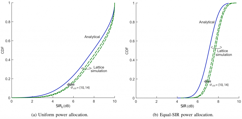
Let us now contrast the analytical expressions (computable instantaneously and exactly, and valid for arbitrary topologies, but asymptotic in the shadowing strength) with some Monte-Carlo simulations (lengthy, noisy, and bug-prone, but for precise shadowing strengths and topologies).
First, we simulate a 500-cell hexagonal lattice with  ,
,  and . Figs. 1a-1b compare the simulations for
  –
– dB with the analysis. The behaviors with these typical outdoor values of are well represented by the analysis and, as it turns out, in rigidly homogeneous networks such as this one is where the gap is largest.
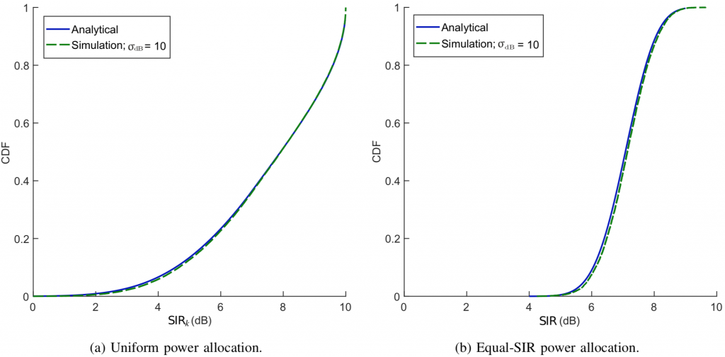
For a more irregular deployment, let us next consider a network whose BSs are uniformly distributed. BSs (500 on average) are dropped around a central one of interest. For each network snapshot, users are then uniformly dropped until of them are served by the central BS. As before, ,  and
and  . Figs. 2a-2b compare the simulations for
  dB with the analysis, and the agreement is now complete. The simulated average spectral efficiency with a uniform power allocation is
  b/s/Hz/user while (2) gives
  b/s/Hz/user.
The analysis presented in this post is not without limitations, chiefly the absence of noise and pilot contamination. However, as argued in [1], there is a broad operating range ( –
– with very conservative premises) where these effects are rather minor, and the analysis is hence applicable.
[1] G. George, A. Lozano, M. Haenggi, “Massive MIMO forward link analysis for cellular networks,” arXiv:1811.00110, 2018.
[2] T. Marzetta, E. Larsson, H. Yang, and H. Ngo, Fundamentals of Massive MIMO. Cambridge University Press, 2016.
[3] H. Yang and T. L. Marzetta, “A macro cellular wireless network with uniformly high user throughputs,” IEEE Veh. Techn. Conf. (VTC’14), Sep. 2014.
Thank you Respected Sir for sharing. Very insightful.
Sir, can we use the UL channel estimates in the DL Massive MIMO system based on TDD protocol. I mean whether exact channel estimation expressions can we use in calculating DL spectral efficiency?
Yes, you can use the same estimates, but the spectral efficiency expressions will look different. You can find expressions in textbooks such as “Fundamentals of Massive MIMO” and “Massive MIMO Networks” (http://massivemimobook.com)
Thanks, Sir.
Sir, the expression 4.39 in (http://massivemimobook.com) is using UL channel estimates?
(http://massivemimobook.com/)
No, not necessarily. It depends on the true channels and the precoding vectors. In practice, the precoding vectors will likely be computed using UL channel estimates, but any selection is supported by the theorem.
Thanks very much Sir.
Sir,
The DL spectral efficiency for massive MIMO with M-MMSE precoding and pilot reuse factor=4, the number of antennas M=100 and K varies from 4 to 20 when I plotted with the help of the code provided by you in (http://massivemimobook.com/). All the other parameter is same as used in the book.
Sir, for K>16 why spectral efficiency decreases slightly…is it due to a decrease in SINR and Pre-log factor? SINR decrease due to pilot contamination for K>16?
I believe the issue is that there is too much interference and too much resources are used for pilot signaling. I don’t think pilot contamination is the main issue in this scenario. I recommend you to read Section 7.2.2 Scheduling, since it discusses these things.
Thanks very much, sir for recommending Section 7.2.2