One reason for why capacity lower bounds are so useful is that they are accurate proxies for link-level performance with modern coding. But this fact, well known to information and coding theorists, is often contested by practitioners. I will discuss some possible reasons for that here.

The recipe is to compute the capacity bound, and depending on the code blocklength, add a dB or a few, to the required SNR. That gives the link performance prediction. The coding literature is full of empirical results, showing how far from capacity a code of a given block length is for the AWGN channel, and this gap is usually not extremely different for other channel models – although, one should always check this.

But there are three main caveats with this:

1. First, the capacity bound, or the “SINR” that it often contains, must be information-theoretically correct. A great deal of papers get this wrong. Emil explained in his blog post last week some common errors. The recommended approach is to map the channel onto one of the canonical cases in Figure 2.9 in Fundamentals of Massive MIMO, verify that the technical conditions are satisfied, and use the corresponding formula.
2. When computing expressions of the type E[log(1+”SINR”)], then the average should be taken over all quantities that are random within the duration of a codeword. Typically, this means averaging over the randomness incurred by the noise, channel estimation errors, and in many cases the small-scale fading. All other parameters must be kept fixed. Typically, user positions, path losses, shadow fading, scheduling and pilot assignments, are fixed, so the expectation is conditional on those. (Yet, the interference statistics may vary substantially, if other users are dropping in and out of the system.) This in turn means that many “drops” have to be generated, where these parameters are drawn at random, and then CDF curves with respect to that second level of randomness needs be computed (numerically).Think of the expectation E[log(1+”SINR”)] as a “link simulation”. Every codeword sees many independent noise realizations, and typically small-scale fading realizations, but the same realization of the user positions. Also, often, neat (and tight) closed-form bounds on E[log(1+”SINR”)] are available.
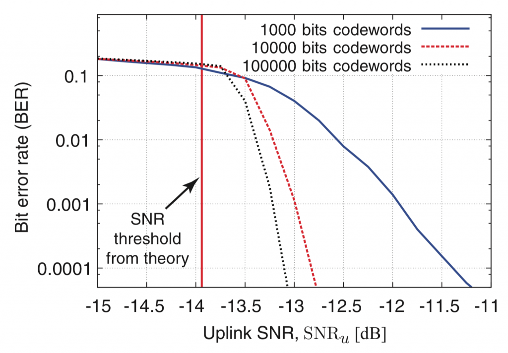
3. Care is advised when working with relatively short blocks (less than a few hundred bits) and at rates close to the constrained capacity with the foreseen modulation format. In this case, many of the “standard” capacity bounds become overoptimistic.As a rule of thumb, compare the capacity of an AWGN channel with the constrained capacity of the chosen modulation at the spectral efficiency of interest, and if the gap is small, the capacity bounds will be useful. If not, then reconsider the choice of modulation format! (See also homework problem 1.4.)

How far are the bounds from the actual capacity typically? Nobody knows, but there are good reasons to believe they are extremely close. Here (Figure 1) is a nice example that compares a decoder that uses the measured channel likelihood, instead of assuming a Gaussian (which is implied by the typical bounding techniques). From correspondence with one of the authors: “The dashed and solid lines are the lower bound obtained by Gaussianizing the interference, while the circles are the rate achievable by a decoder exploiting the non-Gaussianity of the interference, painfully computed through days-long Monte-Carlo. (This is not exactly the capacity, because the transmit signals here are Gaussian, so one could deviate from Gaussian signaling and possibly do slightly better — but the difference is imperceptible in all the experiments we’ve done.)”

Concerning Massive MIMO and its capacity bounds, I have met for a long time with arguments that these capacity formulas aren’t useful estimates of actual performance. But in fact, they are: In one simulation study we were less than one dB from the capacity bound by using QPSK and a standard LDPC code (albeit with fairly long blocks). This bound accounts for noise and channel estimation errors. Such examples are in Chapter 1 of Fundamentals of Massive MIMO, and also in the ten-myth paper:

(I wrote the simulation code, and can share it, in case anyone would want to reproduce the graphs.)

So in summary, while capacity bounds are sometimes done wrong; when done right they give pretty good estimates of actual link performance with modern coding.

(With thanks to Angel Lozano for discussions.)