Category Archives: Commentary

What Happens When Arrays Become Physically Large?

Massive MIMO is all about using large arrays to transmit narrow beams, thereby increasing the received signal power and enabling spatial multiplexing of signals in different directions. Importantly, the words “large” and “massive” have relative meanings in this context: they refer to having many transceiver chains, which leads to many more spatial degrees of freedom in the beamforming design than in previous cellular technologies. However, the physical sizes of the 5G Massive MIMO arrays that are being deployed are similar to previous base station equipment. The reason is that the number of radiating elements is roughly the same and this is what determines the physical size.

What if we would deploy physically large arrays?

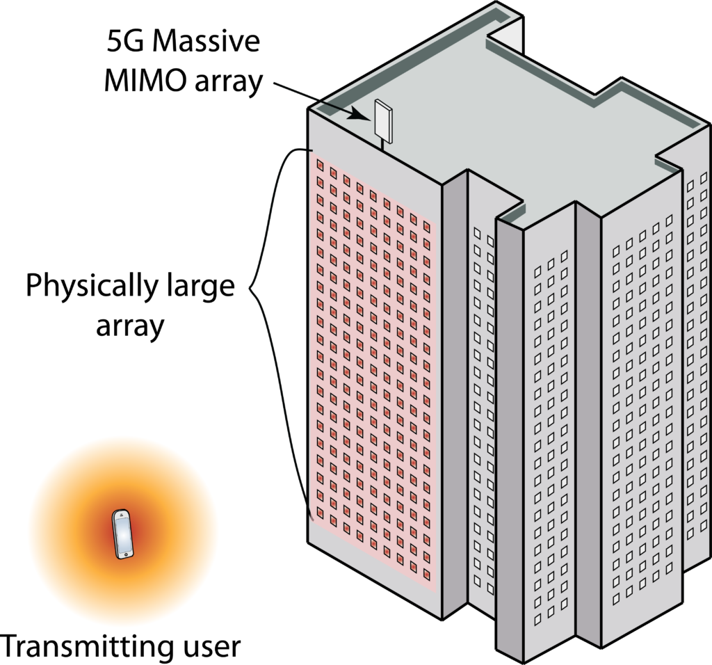
Since base station arrays are deployed at elevated places, many tens of meters from the users, 5G antenna arrays will look small from the viewpoint of the user. This situation might change in the future, when moving beyond 5G. Suppose we would cover the entire facade of a building with antennas, as illustrated in Figure 1, then the array would be physically large, not only feature a large number of transceiver chains.

Figure 1: A 5G Massive MIMO array has many antennas but is not physically large. This blog post considers physically large arrays that might be deployed over an entire building.

There are unusual wireless propagation phenomena that occur in such deployments and these have caught my attention in recent years. A lot of research papers on Massive MIMO consider the asymptotic regime where the number of antennas (transceiver chains) goes to infinity, but the channel models that are being used break down asymptotically. For example, the received signal power goes to infinity although the transmitted power is finite, which is physically impossible.

This inconsistency was a reason for why I didn’t jump onto the Massive MIMO train when it took off in 2010, but waited until I realized that Marzetta’s mind-blowing asymptotic results are also applicable in many practical situations. For example, if the users are at least ten meters away from the base station, we can make use of thousands of antennas before any inconsistencies arise. The asymptotic issues have been stuck in my mind ever since but now I have finally found the time and tools needed to characterize the true asymptotic behaviors.

Three important near-field characteristics

Three phenomena must be properly modeled when the user is close to a physically large array, which we call the array’s near-field. These phenomena are:

  1. The propagation distance varies between the different antennas in the array.
  2. The antennas are perceived to have different effective areas since they are observed from different angles.
  3. The signal losses due to polarisation mismatch vary due to the different angles.

Wireless propagation channels have, of course, always been determined by the propagation distances, effective antenna areas, and polarisation losses. However, one can normally make the approximation that they are equal for all antennas in the array. In our new paper “Power Scaling Laws and Near-Field Behaviors of Massive MIMO and Intelligent Reflecting Surfaces“, we show that all three conditions must be properly modeled to carry out an accurate asymptotic study. The new formulas that we present are confirming the intuition that the part of the array that is closest to the user is receiving more power than the parts that are further away. As the array grows infinitely large, the outer parts receive almost nothing and the results comply with fundamental physics, such as the law of conservation of energy.

You might have heard about the Fraunhofer distance, which is the wavelength-dependent limit between the near-field and far-field of a single antenna. This distance is not relevant in our context since we are not considering the radiative behaviors that occur close to an antenna, but the geometric properties of a large array. We are instead studying the array’s near-field, when the user perceives an electrically large array. The result is wavelength-independent and occurs approximately when the propagation distance is shorter than the widest dimension of the array. This is when one must take the three properties above into account to get accurate results. Note that it is not the absolute size of the array that matters but how large it is compared to the field-of-view of the user.

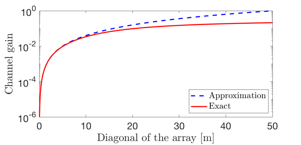
Figure 2 illustrates this property by showing the channel gain (i.e., the fraction of the transmitted power that is received) in a setup with an isotropic transmit antenna that is 10 m from the center of a square array. The diagonal of the array is shown on the horizontal axis. The solid red curve is computed using our new accurate formula, while the blue dashed curve is based on the conventional far-field approximation. The curves are overlapping until the diagonal is 10 m (same as the propagation distance). The difference increases rapidly when the array becomes larger (notice the logarithmic scale on the vertical axis). When the diagonal is 50 m, the approximation errors are extreme: the channel gain surpasses 1, which means that more power is received than was transmitted.

Figure 2: The channel gain when transmitting from a user that is 10 m from a square array. The conventional far-field approximation is accurate until the array becomes so large that one must take the three near-field characteristics into account.

There are practical applications

There are two ongoing lines of research where the new near-field results and insights are useful, both to consolidate the theoretical understanding and from a practical perspective.

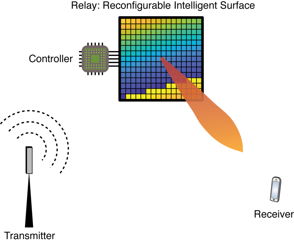
One example is the physically large and dense Massive MIMO arrays which are being called large intelligent surfaces and holographic MIMO. These names are utilized to distinguish the analysis from the physically small Massive MIMO products that are now being deployed in 5G. Another example is the “passive” metasurface-based arrays that are being called reconfigurable intelligent surfaces and intelligent reflecting surfaces. These are arrays of scattering elements that can be configured to scatter an incoming signal from a transmitter towards a receiver.

We are taking a look at both of these areas in the aforementioned paper. In fact, the reason why we initiated the research last year is that we wanted to understand how to compare the asymptotic behaviors of the two technologies, which exhibit different power scaling laws in the far-field but converge to similar limits in the array’s near-field.

If you would like to learn more, I recommend you to read the paper and play around with the simulation code that you can find on GitHub.

Chasing Data Rate Records

5G networks are supposed to be fast, to provide higher data rates than ever before. While indoor experiments have demonstrated huge data rates in the past, this has been the year where the vendors are competing in setting new data rate records in real deployments.

Nokia achieved 4.7 Gbps in an unnamed carrier’s cellular network in the USA in May 2020. This was achieved by dual connectivity where a user device simultaneously used 800 MHz of mmWave spectrum in 5G and 40 MHz of 4G spectrum.

The data rate with the Nokia equipment was higher than the 4.3 Gbps that Ericsson demonstrated in February 2020, but they “only” used 800 MHz of mmWave spectrum. While there are no details on how the 4.7 Gbps was divided between the mmWave and LTE bands, it is likely that Ericsson and Nokia achieved roughly the same data rate over the mmWave bands. The main new aspect was rather the dual connectivity between 4G and 5G.

The high data rates in these experiments are enabled by the abundant spectrum, while the spectral efficiency is only 5.4 bps/Hz. This can be achieved by 64-QAM modulation and high-rate channel coding, a combination of modulation and coding that was available already in LTE. From a technology standpoint, I am more impressed by reports of 3.7 Gbps being achieved over only 100 MHz of bandwidth, because then the spectral efficiency is 37 bps/Hz. That can be achieved in conventional sub-6 GHz bands which have better coverage and, thus, a more consistent 5G service quality.

Reconfigurable Intelligent Surfaces: The Resurrection of Relaying

When I started my research career in 2007, relaying was a very popular topic. It was part of the broader area of cooperative communications, where the communication between the transmitter and the receiver is aided by other nodes that are located in between. This could be anything between a transparent relay that retransmits the signal that reaches it after amplification in the analog domain (so-called amplify-and-forward), to a regenerative relay to processes and optimizes the signal in the digital baseband before retransmission.

There is a large number of different relaying protocols and information theory that underpins the technology. Relaying is supported by many wireless standards but has not become a major commercial success, possibly because the deployment of “pico-cells” is more attractive to network operators looking for improved local-area coverage.

Is relaying is a technology whose time has come?

A resurrection of the relaying topic can be observed in the beyond 5G era. Many researchers are considering a particular kind of relays being called a reconfigurable intelligent surface (RIS), intelligent reflecting surface, or software-controlled metasurface. Despite the different names and repeated claims of RIS being something fundamentally new, it is clearly a relaying technology. An RIS is a node that receives the signal from the transmitter and then re-radiates it with controllable time-delays. An RIS consists of many small elements that can be assigned different time-delays and thereby synthesize the scattering behavior of an arbitrarily-shaped object of the same size. This feature can, for instance, be used to beamform the signal towards the receiver as shown in the figure below.

Using the conventional terminology, an RIS is a full-duplex transparent relay since the signals are processed in the analog domain and the surface can receive and re-transmit waves simultaneously. The protocol resembles classical amplify-and-forward, except that the signals are not amplified. The main idea is instead to have a very large surface area so it can then capture an unusually large fraction of the signal power and use the large aperture to re-radiate narrow beams.

Conventional full-duplex relays suffer from loop-back interference, where the amplified signals leak into the yet-to-be-amplified signals in the relay. This issue is avoided in the RIS technology but is replaced by several other fundamental research challenges. In our new paper “Reconfigurable Intelligent Surfaces: Three Myths and Two Critical Questions“, we are pointing out the two most burning research questions that must be answered. We are also debunking three myths surrounding the RIS, whereof one is related to relaying.

I have also recorded a YouTube video explaining the fundamentals:

Many Applications for Correlated Fading Models

The channel fading in traditional frequency bands (below 6 GHz) is often well described by the Rayleigh fading model, at least in non-line-of-sight scenarios. This model says that the channel coefficient between any transmit antenna and receive antenna is complex Gaussian distributed, so that its magnitude is Rayleigh distributed.

If there are multiple antennas at the transmitter and/or receiver, then it is common to assume that different pairs of antennas are subject to independent and identically distributed (i.i.d.) fading. This model is called i.i.d. Rayleigh fading and dominates the academic literature to such an extent that one might get the impression that it is the standard case in practice. However, it is rather the other way around: i.i.d. Rayleigh fading only occurs in very special cases in practice, such as having a uniform linear array with half-wavelength-spaced isotropic antennas that is deployed in a rich scattering environment where the multi-paths are uniformly distributed in all directions. If one would remove any of these very specific assumptions then the channel coefficients will become mutually correlated. I covered the basics of spatial correlation in a previous blog post.

In reality, the channel fading will always be correlated

Some reasons for this are: 1) planar arrays exhibit correlation along the diagonals, since not all adjacent antennas can be half-wavelength-spaced; 2) the antennas have non-isotropic radiation patterns; 3) there will be more multipath components from some directions than from other directions.

With this in mind, I have dedicated a lot of my work to analyzing MIMO communications with correlated Rayleigh fading. In particular, our book “Massive MIMO networks” presents a framework for analyzing multi-user MIMO systems that are subject to correlated fading. When we started the writing, I thought spatial correlation was a phenomenon that was important to cover to match reality but would have a limited impact on the end results. I have later understood that spatial correlation is fundamental to understand how communication systems work. In particular, the modeling of spatial correlation changes the game when it comes to pilot contamination: it is an entirely negative effect under i.i.d. Rayleigh fading models, while a proper analysis based on spatial correlation reveals that one can sometimes benefit from purposely assigning the same pilots to users and then separate them based on their spatial correlation properties.

Future applications for spatial correlation models

The book “Massive MIMO networks” presents a framework for channel estimation and computation of achievable rates with uplink receive combining and downlink precoding for correlated Rayleigh fading channels. Although the title of the book implies that it is about Massive MIMO, the results apply to many beyond-5G research topics. Let me give two concrete examples:

  1. Cell-free Massive MIMO: In this topic, many geographically distributed access points are jointly serving all the users in the network. This is essentially a single-cell Massive MIMO system where the access points can be viewed as the distributed antennas of a single base station. The channel estimation and computation of achievable rates can be carried out as described “Massive MIMO networks”. The key differences are instead related to which precoding/combining schemes that are considered practically implementable and the reuse of pilots within a cell (which is possible thanks to the strong spatial correlation).
  2. Extremely Large Aperture Arrays: There are other names for this category, such as holographic MIMO, large intelligent surfaces, and ultra-massive MIMO. The new terminologies are used to indicate the use of co-located arrays that are much larger (in terms of the number of antennas and the physical size) than what is currently considered by the industry when implementing Massive MIMO in 5G. In this case, the spatial correlation matrices must be computed differently than described in “Massive MIMO networks”, for example, to take near-field effects and shadow fading variations into consideration. However, once the spatial correlation matrices have been computed, then the same framework for channel estimation and computation of achievable rates is applicable.

The bottom line is that we can analyze many new exciting beyond-5G technologies by making use of the analytical frameworks developed in the past decade. There is no need to reinvent the wheel but we should reuse as much as possible from previous research and then focus on the novel components. Spatial correlation is something that we know how to deal with and this must not be forgotten.

How “Massive” are the Current Massive MIMO Base Stations?

I have written earlier that the Massive MIMO base stations that have been deployed by Sprint, and other operators, are very capable from a hardware perspective. They are equipped with 64 fully digital antennas, have a rather compact form factor, and can handle wide bandwidths in the 2-3 GHz bands. These facts are supported by documentation that can be accessed in the FCC databases.

However, we can only guess what is going on under the hood – what kind of signal processing algorithms have been implemented and how they perform compared to ideal cases described in the academic literature. Erik G. Larsson recently wrote about how Nokia improved its base station equipment via a software upgrade. Are the latest base stations now as “Massive MIMO”-like as they can become?

My guess is that there is still room for substantial improvements. The following joint video from Sprint and Nokia explains how their latest base stations are running 4G and 5G simultaneously on the same 64-antenna base station and are able to multiplex 16 layers.

This is the highest number of multiuser MIMO layers achieved in the US” according to the speaker. But if you listen carefully, they are actually sending 8 layers on 4G and 8 layers 5G. That doesn’t sum up to 16 layers! The things called layers in 3GPP are signals that are transmitted simultaneously in the same band, but with different spatial directivity. In every part of the spectrum, there are only 8 spatially multiplexed layers in the setup considered in the video.

It is indeed impressive that Sprint can simultaneously deliver around 670 Mbit/s per user to 4 users in the cell, according to the video. However, the spectral efficiency per cell is “only” 22.5 bit/s/Hz, which can be compared to the 33 bit/s/Hz that was achieved in real-world trials by Optus and Huawei in 2017.

Both numbers are far from the world record in spectral efficiency of 145.6 bit/s/Hz that was achieved in a lab environment in Bristol, in a collaboration between the universities in Bristol and Lund. Although we cannot expect to reach those numbers in real-world urban deployments, I believe we can reach higher numbers by building 64-antenna arrays with a different form factor: long linear arrays instead of compact square panels. Since most users are separable in terms of having different azimuth angles to the base station, it will be easier to separate them by sending “narrower” beams in the horizontal domain.

Record 5G capacity via software upgrade!

In the news: Nokia delivers record 5G capacity gains through a software upgrade.   No surprise!  We expected, years ago, this would happen.

What does this software upgrade consist of?  I can only speculate.  It is, in all likelihood, more than the usual (and endless) operating system bugfixes we habitually think of as “software upgrades”.   Could it be even something that goes to the core of what massive MIMO is?  Replacing eigen-beamforming with true reciprocity-based beamforming?! Who knows. Replacing maximum-ratio processing with zero-forcing combining?!  Or even more mind-boggling, implementing more sophisticated processing of the sort that has been stuffing the academic journals in the last years? We don’t know!  But it will certainly be interesting to find out at some point, and it seems safe to assume that this race will continue.  

A lot of improvement could be achieved over the baseline canonical massive MIMO processing. One could, for example, exploit fading correlation, develop improved power control algorithms or implement algorithms that learn the propagation environment, autonomously adapt, and predict the channels.  

It might seem that research already squeezed every drop out of the physical layer, but I do not think so.  Huge gains likely remain to be harvested when resources are tight, and especially we are limited by coherence: high carriers means short coherence, and high mobility might mean almost no coherence at all.  When the system is starved of coherence, then even winning a couple of samples on the pilot channel means a lot.  Room for new elegant theory in “closed form”?  Good question. Could sound heartbreaking, but maybe we have to give up on that.  Room for useful algorithms and innovation? Certainly yes.  A lot.  The race will continue.

Towards 6G: Massive MIMO is a Reality—What is Next?

The good side of the social distancing that is currently taking place is that I have spent more time recording video material than usual. For example, I was supposed to give a tutorial entitled “Signal Processing for MIMO Communications Beyond 5G” at ICASSP 2020 in Barcelona in the beginning of May. This conference has now turned into an online event with free registration. Hence, anyone can attend the tutorial that I am giving together with Jiayi Zhang from Beijing Jiaotong University. We have prerecorded the presentations, which will be broadcasted to the conference attendees on May 4, but will be available for live discussions in between each video segment.

As a teaser for this tutorial, I have uploaded the 30 minute introduction to YouTube:

In this video, I explain what Massive MIMO is, what role it plays in 5G, why there will be a large gap between the theoretical performance and what is achieved in practice, and what might come next. In particular, I explain my philosophy regarding 6G research.

The remaining 2.5 hours of the tutorial will only be available from ICASSP. I hope to meet you online on May 4!