If you are an academic physical-layer researcher, like me, you might be used to treating the base station as a single unit that takes a digital data signal as input and then outputs an electromagnetic radio wave (or the opposite in the uplink). The reality is quite different, or at least it used to be.
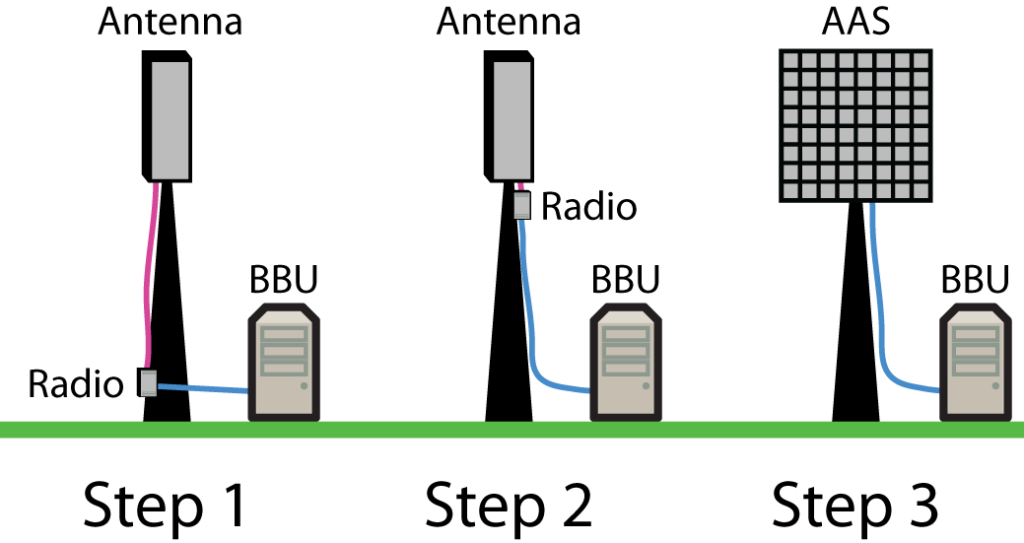
A traditional base station consists of three main components: a baseband unit (BBU) that takes care of digital signal processing, a radio unit that creates the analog radio-frequency (RF) signal, and a passive antenna that emits the RF signals with a constant radiation pattern. Due to the size and weight constraints of masts and towers, the radio and BBU are deployed underneath and there is a long RF feeder cable between the antenna and radio, resulting in substantial power losses. This is illustrated as “Step 1” in the figure below. A single BBU can support multiple radios that are deployed on the same site, which might cover different frequency bands or cell sectors (this is not illustrated).
Figure: The evolution of base station technology has gone through three main steps. In Step 1, the antenna is in the mast while the radio and BBU are underneath. The short blue cable sends digital baseband signals while the long purple cable sends analog RF signals. In Step 2, the radio is next to the antenna, so the purple RF cable is shorter. In Step 3, the antenna and radio are integrated into a single box. Multiple antennas and radios can be contained in the same box, which is called an AAS. The BBU can either be located underneath the AAS or “in the cloud”.
Now when the radio hardware has reduced in size, it is common to use remote radio units that are deployed in the tower, close to the antenna instead of close to the BBU. This is denoted as “Step 2” in the figure above and became common in the 4G era. Only a short RF feeder cable is then needed, while an optical fiber can be drawn from the BBU to the radio. The next step in the development is active antennas that integrate the antenna and radio into a single unit. There are many types of active antennas, from single-antenna units with constant radiation patterns to Massive MIMO antennas that adapt the radiation patterns by beamforming. To distinguish these things, the term advanced antenna system (AAS) is being used in the industry to refer to active Massive MIMO antenna arrays. This setup is denoted as “Step 3” in the figure and is becoming the dominating approach in the 5G era. To limit the capacity of the optical fiber between the AAS and BBU, an AAS might perform a limited set of baseband processing to compress/decompress the signals.
In summary, the latest radio-integrated active antennas are quite similar to what physical-layer researchers have been imaging for a while: A single unit that takes digital signals as input and emits an RF signal. Small cells can even include the BBU in the active antenna, while macro cell deployments purposely keep the BBU separate so it can be shared between multiple active antennas (it can even be moved to a nearby “cloud” computer). The advent of AAS technology is a key enabling factor for Massive MIMO deployment; a single box with 64 antennas and 64 radios can be made rather compact, while a deployment with 64 separate antenna boxes, 64 separate radio units, and an equal number of cables wouldn’t make practical sense.
I received an email in late August 2019 from my former boss at KTH, Professor Peter Händel. He had been working for many years on the modeling of hardware imperfections in wireless transceivers. Our research journeys had recently crossed since he had written several papers on the modeling of imperfections in MIMO transmitters and their impact on communication performance. I have been working on similar things but using far less sophisticated models.
The essence of the email was that he wanted us to write a paper together, but the circumstances came as a chock. Peter had been sick for a while and it turned out to be a terminal illness. He asked me to finalize a manuscript that he had initiated. I agreed and we exchanged a few emails but just as I and my postdoc were about to begin the editing of Peter’s manuscript, he passed away on September 15, 2019.
Impact of Backward Crosstalk in MIMO Transmitters
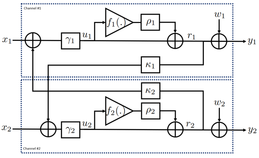
The manuscript considers a type of hardware impairment called backward crosstalk. It can be a major issue in the design of multi-antenna transmitters, but is generally overlooked by communication engineers. The issue arises when you build an antenna-integrated radio, for example, a Massive MIMO array with many antenna elements, power amplifiers, and radio-signal generators in a compact box. In this case, the output signal from one power amplifier will leak into the inputs of the neighboring power amplifiers. Even if the leakage is small in relative terms, it can still have a non-negligible impact since the output power of an amplifier is much higher than the input power. A small fraction of a large power value can still be rather large. In addition to this kind of backward crosstalk between amplifiers, there is also forward crosstalk in practice but it can be neglected for the very same reason.
This figure from the figure illustrates how the output signals r1, r2 from two neighboring power amplifiers are leaking into each other. The variables κ1, κ2 are representing the strength of this backward crosstalk.
We managed to finalize the manuscript, thanks to the excellent work by my postdoc Özlem Tuğfe Demir. The paper is now available:
The paper considers a system model containing backward crosstalk, as well as, power amplifier non-linearities and transmitter noise. We characterize the performance both at the transmitter side (the normalized mean-squared error) and at the receiver side (the spectral efficiency). In turns out that optimization based on these two metrics can lead to very different transmission strategies; from a spectral efficiency perspective, one can transmit at higher power and accept a higher level of distortion since the desired signal power is also growing. In the paper, we also demonstrate how the precoding can be adapted to partially compensate for the crosstalk.
This paper is just a first step towards modeling real hardware imperfections that are normally ignored in academia or lumped together into a single additive term characterized by the error-vector magnitude. In the last emails I received from Peter, he expressed his view that there is a lot of open problems to solve at the interface between proper modeling of communication hardware and the design of signal processing schemes. I agree with him and encourage anyone who is looking for open problems on MIMO communications to have a closer look at his final papers on this topic:
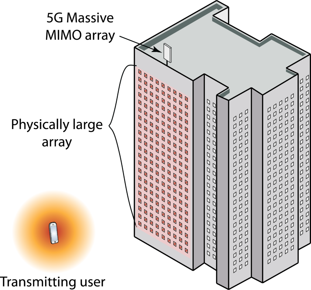
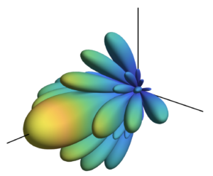
Massive MIMO is all about using large arrays to transmit narrow beams, thereby increasing the received signal power and enabling spatial multiplexing of signals in different directions. Importantly, the words “large” and “massive” have relative meanings in this context: they refer to having many transceiver chains, which leads to many more spatial degrees of freedom in the beamforming design than in previous cellular technologies. However, the physical sizes of the 5G Massive MIMO arrays that are being deployed are similar to previous base station equipment. The reason is that the number of radiating elements is roughly the same and this is what determines the physical size.
What if we would deploy physically large arrays?
Since base station arrays are deployed at elevated places, many tens of meters from the users, 5G antenna arrays will look small from the viewpoint of the user. This situation might change in the future, when moving beyond 5G. Suppose we would cover the entire facade of a building with antennas, as illustrated in Figure 1, then the array would be physicallylarge, not only feature a large number of transceiver chains.
Figure 1: A 5G Massive MIMO array has many antennas but is not physically large. This blog post considers physically large arrays that might be deployed over an entire building.
There are unusual wireless propagation phenomena that occur in such deployments and these have caught my attention in recent years. A lot of research papers on Massive MIMO consider the asymptotic regime where the number of antennas (transceiver chains) goes to infinity, but the channel models that are being used break down asymptotically. For example, the received signal power goes to infinity although the transmitted power is finite, which is physically impossible.
This inconsistency was a reason for why I didn’t jump onto the Massive MIMO train when it took off in 2010, but waited until I realized that Marzetta’s mind-blowing asymptotic results are also applicable in many practical situations. For example, if the users are at least ten meters away from the base station, we can make use of thousands of antennas before any inconsistencies arise. The asymptotic issues have been stuck in my mind ever since but now I have finally found the time and tools needed to characterize the true asymptotic behaviors.
Three important near-field characteristics
Three phenomena must be properly modeled when the user is close to a physically large array, which we call the array’s near-field. These phenomena are:
The propagation distance varies between the different antennas in the array.
The antennas are perceived to have different effective areas since they are observed from different angles.
The signal losses due to polarisation mismatch vary due to the different angles.
Wireless propagation channels have, of course, always been determined by the propagation distances, effective antenna areas, and polarisation losses. However, one can normally make the approximation that they are equal for all antennas in the array. In our new paper “Power Scaling Laws and Near-Field Behaviors of Massive MIMO and Intelligent Reflecting Surfaces“, we show that all three conditions must be properly modeled to carry out an accurate asymptotic study. The new formulas that we present are confirming the intuition that the part of the array that is closest to the user is receiving more power than the parts that are further away. As the array grows infinitely large, the outer parts receive almost nothing and the results comply with fundamental physics, such as the law of conservation of energy.
You might have heard about the Fraunhofer distance, which is the wavelength-dependent limit between the near-field and far-field of a single antenna. This distance is not relevant in our context since we are not considering the radiative behaviors that occur close to an antenna, but the geometric properties of a large array. We are instead studying the array’s near-field, when the user perceives an electrically large array. The result is wavelength-independent and occurs approximately when the propagation distance is shorter than the widest dimension of the array. This is when one must take the three properties above into account to get accurate results. Note that it is not the absolute size of the array that matters but how large it is compared to the field-of-view of the user.
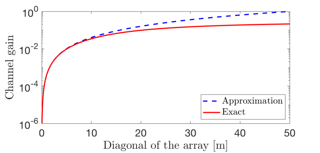
Figure 2 illustrates this property by showing the channel gain (i.e., the fraction of the transmitted power that is received) in a setup with an isotropic transmit antenna that is 10 m from the center of a square array. The diagonal of the array is shown on the horizontal axis. The solid red curve is computed using our new accurate formula, while the blue dashed curve is based on the conventional far-field approximation. The curves are overlapping until the diagonal is 10 m (same as the propagation distance). The difference increases rapidly when the array becomes larger (notice the logarithmic scale on the vertical axis). When the diagonal is 50 m, the approximation errors are extreme: the channel gain surpasses 1, which means that more power is received than was transmitted.
Figure 2: The channel gain when transmitting from a user that is 10 m from a square array. The conventional far-field approximation is accurate until the array becomes so large that one must take the three near-field characteristics into account.
There are practical applications
There are two ongoing lines of research where the new near-field results and insights are useful, both to consolidate the theoretical understanding and from a practical perspective.
One example is the physically large and dense Massive MIMO arrays which are being called large intelligent surfaces and holographic MIMO. These names are utilized to distinguish the analysis from the physically small Massive MIMO products that are now being deployed in 5G. Another example is the “passive” metasurface-based arrays that are being called reconfigurable intelligent surfaces and intelligent reflecting surfaces. These are arrays of scattering elements that can be configured to scatter an incoming signal from a transmitter towards a receiver.
We are taking a look at both of these areas in the aforementioned paper. In fact, the reason why we initiated the research last year is that we wanted to understand how to compare the asymptotic behaviors of the two technologies, which exhibit different power scaling laws in the far-field but converge to similar limits in the array’s near-field.
Since the pandemic made it hard to travel over the world, several open online seminar series have appeared with focus on different research topics. The idea seems to be to give researchers a platform to attend talks by international experts and enable open discussions.
There is a “One World Signal Processing Seminar Series” series, which has partially considered topics on multi-antenna communications. I want to highlight one such seminar. Professor Wei Yu (University of Toronto) is talking about Machine Learning for Massive MIMO Communications. The video contains a 45 minute long presentation plus another 30 minutes where questions are being answered.
When I started my research career in 2007, relaying was a very popular topic. It was part of the broader area of cooperative communications, where the communication between the transmitter and the receiver is aided by other nodes that are located in between. This could be anything between a transparent relay that retransmits the signal that reaches it after amplification in the analog domain (so-called amplify-and-forward), to a regenerative relay to processes and optimizes the signal in the digital baseband before retransmission.
There is a large number of different relaying protocols and information theory that underpins the technology. Relaying is supported by many wireless standards but has not become a major commercial success, possibly because the deployment of “pico-cells” is more attractive to network operators looking for improved local-area coverage.
Is relaying is a technology whose time has come?
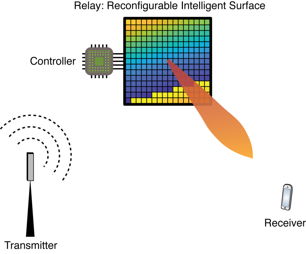
A resurrection of the relaying topic can be observed in the beyond 5G era. Many researchers are considering a particular kind of relays being called a reconfigurable intelligent surface (RIS), intelligent reflecting surface, or software-controlled metasurface. Despite the different names and repeated claims of RIS being something fundamentally new, it is clearly a relaying technology. An RIS is a node that receives the signal from the transmitter and then re-radiates it with controllable time-delays. An RIS consists of many small elements that can be assigned different time-delays and thereby synthesize the scattering behavior of an arbitrarily-shaped object of the same size. This feature can, for instance, be used to beamform the signal towards the receiver as shown in the figure below.
Using the conventional terminology, an RIS is a full-duplex transparent relay since the signals are processed in the analog domain and the surface can receive and re-transmit waves simultaneously. The protocol resembles classical amplify-and-forward, except that the signals are not amplified. The main idea is instead to have a very large surface area so it can then capture an unusually large fraction of the signal power and use the large aperture to re-radiate narrow beams.
Conventional full-duplex relays suffer from loop-back interference, where the amplified signals leak into the yet-to-be-amplified signals in the relay. This issue is avoided in the RIS technology but is replaced by several other fundamental research challenges. In our new paper “Reconfigurable Intelligent Surfaces: Three Myths and Two Critical Questions“, we are pointing out the two most burning research questions that must be answered. We are also debunking three myths surrounding the RIS, whereof one is related to relaying.
I have also recorded a YouTube video explaining the fundamentals:
The channel fading in traditional frequency bands (below 6 GHz) is often well described by the Rayleigh fading model, at least in non-line-of-sight scenarios. This model says that the channel coefficient between any transmit antenna and receive antenna is complex Gaussian distributed, so that its magnitude is Rayleigh distributed.
If there are multiple antennas at the transmitter and/or receiver, then it is common to assume that different pairs of antennas are subject to independent and identically distributed (i.i.d.) fading. This model is called i.i.d. Rayleigh fading and dominates the academic literature to such an extent that one might get the impression that it is the standard case in practice. However, it is rather the other way around: i.i.d. Rayleigh fading only occurs in very special cases in practice, such as having a uniform linear array with half-wavelength-spaced isotropic antennas that is deployed in a rich scattering environment where the multi-paths are uniformly distributed in all directions. If one would remove any of these very specific assumptions then the channel coefficients will become mutually correlated. I covered the basics of spatial correlation in a previous blog post.
In reality, the channel fading will always be correlated
Some reasons for this are: 1) planar arrays exhibit correlation along the diagonals, since not all adjacent antennas can be half-wavelength-spaced; 2) the antennas have non-isotropic radiation patterns; 3) there will be more multipath components from some directions than from other directions.
With this in mind, I have dedicated a lot of my work to analyzing MIMO communications with correlated Rayleigh fading. In particular, our book “Massive MIMO networks” presents a framework for analyzing multi-user MIMO systems that are subject to correlated fading. When we started the writing, I thought spatial correlation was a phenomenon that was important to cover to match reality but would have a limited impact on the end results. I have later understood that spatial correlation is fundamental to understand how communication systems work. In particular, the modeling of spatial correlation changes the game when it comes to pilot contamination: it is an entirely negative effect under i.i.d. Rayleigh fading models, while a proper analysis based on spatial correlation reveals that one can sometimes benefit from purposely assigning the same pilots to users and then separate them based on their spatial correlation properties.
Future applications for spatial correlation models
The book “Massive MIMO networks” presents a framework for channel estimation and computation of achievable rates with uplink receive combining and downlink precoding for correlated Rayleigh fading channels. Although the title of the book implies that it is about Massive MIMO, the results apply to many beyond-5G research topics. Let me give two concrete examples:
Cell-free Massive MIMO: In this topic, many geographically distributed access points are jointly serving all the users in the network. This is essentially a single-cell Massive MIMO system where the access points can be viewed as the distributed antennas of a single base station. The channel estimation and computation of achievable rates can be carried out as described “Massive MIMO networks”. The key differences are instead related to which precoding/combining schemes that are considered practically implementable and the reuse of pilots within a cell (which is possible thanks to the strong spatial correlation).
Extremely Large Aperture Arrays: There are other names for this category, such as holographic MIMO, large intelligent surfaces, and ultra-massive MIMO. The new terminologies are used to indicate the use of co-located arrays that are much larger (in terms of the number of antennas and the physical size) than what is currently considered by the industry when implementing Massive MIMO in 5G. In this case, the spatial correlation matrices must be computed differently than described in “Massive MIMO networks”, for example, to take near-field effects and shadow fading variations into consideration. However, once the spatial correlation matrices have been computed, then the same framework for channel estimation and computation of achievable rates is applicable.
The bottom line is that we can analyze many new exciting beyond-5G technologies by making use of the analytical frameworks developed in the past decade. There is no need to reinvent the wheel but we should reuse as much as possible from previous research and then focus on the novel components. Spatial correlation is something that we know how to deal with and this must not be forgotten.
I have written earlier that the Massive MIMO base stations that have been deployed by Sprint, and other operators, are very capable from a hardware perspective. They are equipped with 64 fully digital antennas, have a rather compact form factor, and can handle wide bandwidths in the 2-3 GHz bands. These facts are supported by documentation that can be accessed in the FCC databases.
However, we can only guess what is going on under the hood – what kind of signal processing algorithms have been implemented and how they perform compared to ideal cases described in the academic literature. Erik G. Larsson recently wrote about how Nokia improved its base station equipment via a software upgrade. Are the latest base stations now as “Massive MIMO”-like as they can become?
My guess is that there is still room for substantial improvements. The following joint video from Sprint and Nokia explains how their latest base stations are running 4G and 5G simultaneously on the same 64-antenna base station and are able to multiplex 16 layers.
“This is the highest number of multiuser MIMO layers achieved in the US” according to the speaker. But if you listen carefully, they are actually sending 8 layers on 4G and 8 layers 5G. That doesn’t sum up to 16 layers! The things called layers in 3GPP are signals that are transmitted simultaneously in the same band, but with different spatial directivity. In every part of the spectrum, there are only 8 spatially multiplexed layers in the setup considered in the video.
It is indeed impressive that Sprint can simultaneously deliver around 670 Mbit/s per user to 4 users in the cell, according to the video. However, the spectral efficiency per cell is “only” 22.5 bit/s/Hz, which can be compared to the 33 bit/s/Hz that was achieved in real-world trials by Optus and Huawei in 2017.
Both numbers are far from the world record in spectral efficiency of 145.6 bit/s/Hz that was achieved in a lab environment in Bristol, in a collaboration between the universities in Bristol and Lund. Although we cannot expect to reach those numbers in real-world urban deployments, I believe we can reach higher numbers by building 64-antenna arrays with a different form factor: long linear arrays instead of compact square panels. Since most users are separable in terms of having different azimuth angles to the base station, it will be easier to separate them by sending “narrower” beams in the horizontal domain.