I wrote this paper to make a single point: the hardware distortion (especially out-band radiation) stemming from transmitter nonlinearities in massive MIMO is a deterministic function of the transmitted signals. One consequence of this is that in most cases of practical relevance, the distortion is correlated among the antennas. Specifically, under line-of-sight propagation conditions this distortion is radiated in specific directions: in the single-user case the distortion is radiated into the same direction as the signal of interest, and in the two-user case the distortion is radiated into two other directions.

The derivation was based on a very simple third-order polynomial model. Questioning that model, or contesting the conclusions? Let’s run WebLab. WebLab is a web-server-based interface to a real power amplifier operating in the lab, developed and run by colleagues at Chalmers University of Technology in Sweden. Anyone can access the equipment in real time (though there might be a queue) by submitting a waveform and retrieving the amplified waveform using a special Matlab function, “weblab.m”, obtainable from their webpages. Since accurate characterization and modeling of amplifiers is a hard nonlinear identification problem, WebLab is a great tool to researchers who want to go beyond polynomial and truncated Volterra-type toy models.

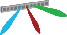
A -spaced uniform linear array with 50 elements beamforms in free space line-of-sight to two terminals at (arbitrarily chosen) angles -9 respectively +34 degrees. A sinusoid with frequency is sent to the first terminal, and a sinusoid with frequency is transmitted to the other terminal. (Frequencies are in discrete time, see the Weblab documentation for details.) The actual radiation diagram is computed numerically: line-of-sight in free space is fairly uncontroversial: superposition for wave propagation applies. However, importantly, the actual amplification all signals is run on actual hardware in the lab.

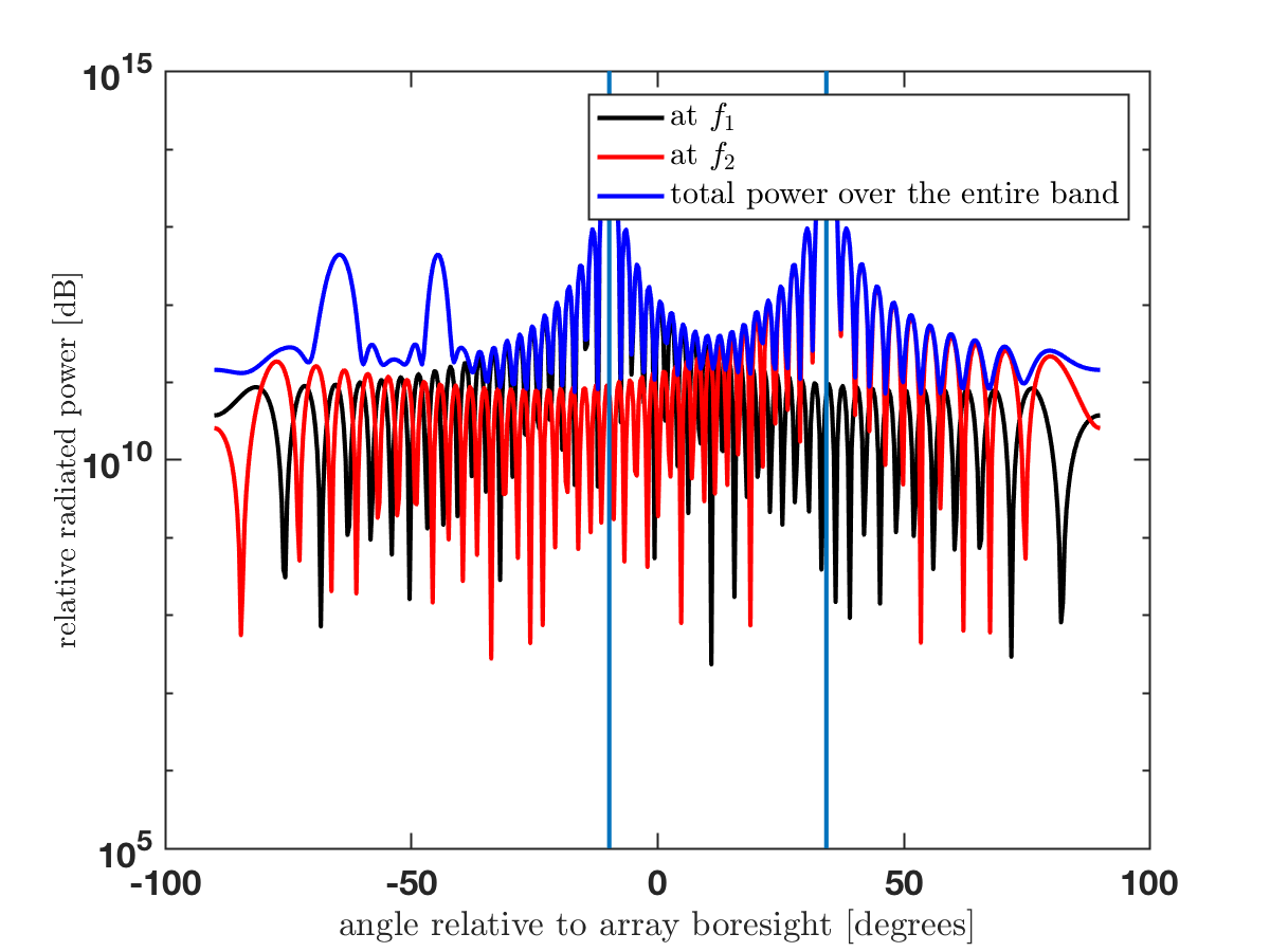
The computed radiation diagram is shown below. (Some lines overlap.) There are two large peaks at -9 and +34 degrees angle, corresponding to the two signals of interest with frequencies and . There are also secondary peaks, at angles approximately -44 and -64 degrees, at frequencies different from respectively . These peaks originate from intermodulation products, and represent the out-band radiation caused by the amplifier non-linearity. (Homework: read the paper and verify that these angles are equal to those predicted by the theory.)

The Matlab code for reproduction of this experiment can be downloaded here.

Last year, I wrote a post about channel hardening. To recap, the achievable data rate of a conventional single-antenna channel varies rapidly over time due to the random small-scale fading realizations, and also over frequency due to frequency-selective fading. However, when you have many antennas at the base station and use them for coherent precoding/combining, the fluctuations in data rate average out; we then say that the channel hardens. One follow-up question that I’ve got several times is:

Can we utilize the channel hardening to estimate the channels less frequently?

Unfortunately, the answer is no. Whenever you move approximately half a wavelength, the multi-path propagation will change each element of the channel vector. The time it takes to move such a distance is called a coherence time. This time is the same irrespectively of how many antennas the base station has and, therefore, you still need to estimate the channel once per coherence time. The same applies to the frequency domain, where the coherence bandwidth is determined by the propagation environment and not the number of antennas.

The following flow-chart shows what need to happen in every channel coherence time:

When you get a new realization (at the top of the flow-chart), you compute an estimate (e.g., based on uplink pilots), then you use the estimate to compute a new receive combining vector and transmit precoding vector. It is when you have applied these vectors to the channel that the hardening phenomena appears; that is, the randomness averages out. If you use maximum ratio (MR) processing, then the random realization h₁ of the channel vector turns into an almost deterministic scalar channel ||h₁||². You can communicate over the hardened channel with gain ||h₁||² until the end of the coherence time. You then start over again by estimating the new channel realization h₂, applying MR precoding/combining again, and then you get ||h₂||² ≈ ||h₁||².

In conclusion, channel hardening appears after coherent combining/precoding has been applied. To maintain a hardened channel over time (and frequency), you need to estimate and update the combining/precoding as often as you would do for a single-antenna channel. If you don’t do that, you will gradually lose the array gain until the point where the channel and the combining/precoding are practically uncorrelated, so there is no array gain left. Hence, there is more to lose from estimating channels too infrequently in Massive MIMO systems than in conventional systems. This is shown in Fig. 10 in a recent measurement paper from Lund University, where you see how the array gain vanishes with time. However, the Massive MIMO system will never be worse than the corresponding single-antenna system.