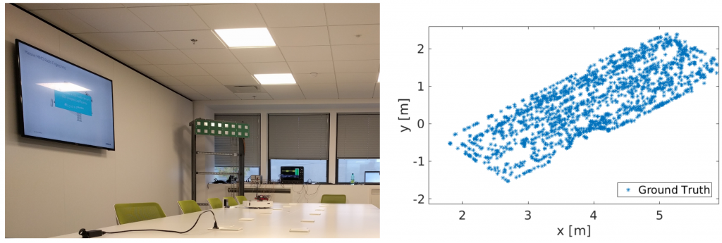
The object of the competition is to design and train an algorithm that can determine the position of a user, based on estimated channel frequency responses between the user and an antenna array. Possible solutions may build on classic algorithms (fingerprinting, interpolation) or machine-learning approaches. Channel vectors from a dataset created with a MIMO channel sounder will be used.
Competing teams should present a poster at the conference, describing their algorithms and experiments.
A $500 USD prize will be awarded to the winning team.
Come listen to Liesbet Van der Perre, Professor at KU Leuven (Belgium) on Monday February 18 at 2.00 pm EST.
She gives a webinar on state-of-the-art circuit implementations of Massive MIMO, and outlines future research challenges. The webinar is based on, among others, this paper.
In more detail the webinar will summarize the fundamental technical contributions to efficient digital signal processing for Massive MIMO. The opportunities and constraints on operating on low-complexity RF and analog hardware chains are clarified. It will explain how terminals can benefit from improved energy efficiency. The status of technology and real-life prototypes will be discussed. Open challenges and directions for future research are suggested.
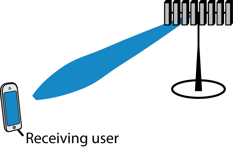
When an antenna array is used to focus a transmitted signal on a receiver, we call this beamforming (or precoding) and we usually illustrate it as shown to the right. This cartoonish illustration is only applicable when the antennas are gathered in a compact array and there is a line-of-sight channel to the receiver.
If we want to deploy very many antennas, as in Massive MIMO, it might be preferable to distribute the antennas over a larger area. One such deployment concept is called Cell-free Massive MIMO. The basic idea is to have many distributed antennas that are transmitting phase-coherently to the receiving user. In other words, the antennas’ signal components add constructively at the location of the user, just as when using a compact array for beamforming. It is therefore convenient to call it beamforming in both cases—algorithmically it is the same thing!
The question is: How can we illustrate the beamforming effect when using a distributed array?
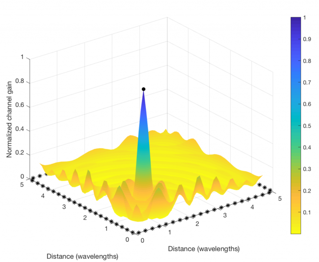
The figure below shows how to do it. I consider a toy example with 80 star-marked antennas deployed along the sides of a square and these antennas are transmitting sinusoids with equal power, but different phases. The phases are selected to make the 80 sine-components phase-aligned at one particular point in space (where the receiving user is supposed to be):
Clearly, the “beamforming” from a distributed array does not give rise to a concentrated signal beam, but the signal amplification is confined to a small spatial region (where the color is blue and the values on the vertical axis are close to one). This is where the signal components from all the antennas are coherently combined. There are minor fluctuations in channel gain at other places, but the general trend is that the components are non-coherently combined everywhere except at the receiving user. (Roughly the same will happen in a rich multipath channel, even if a compact array is used for transmission.)
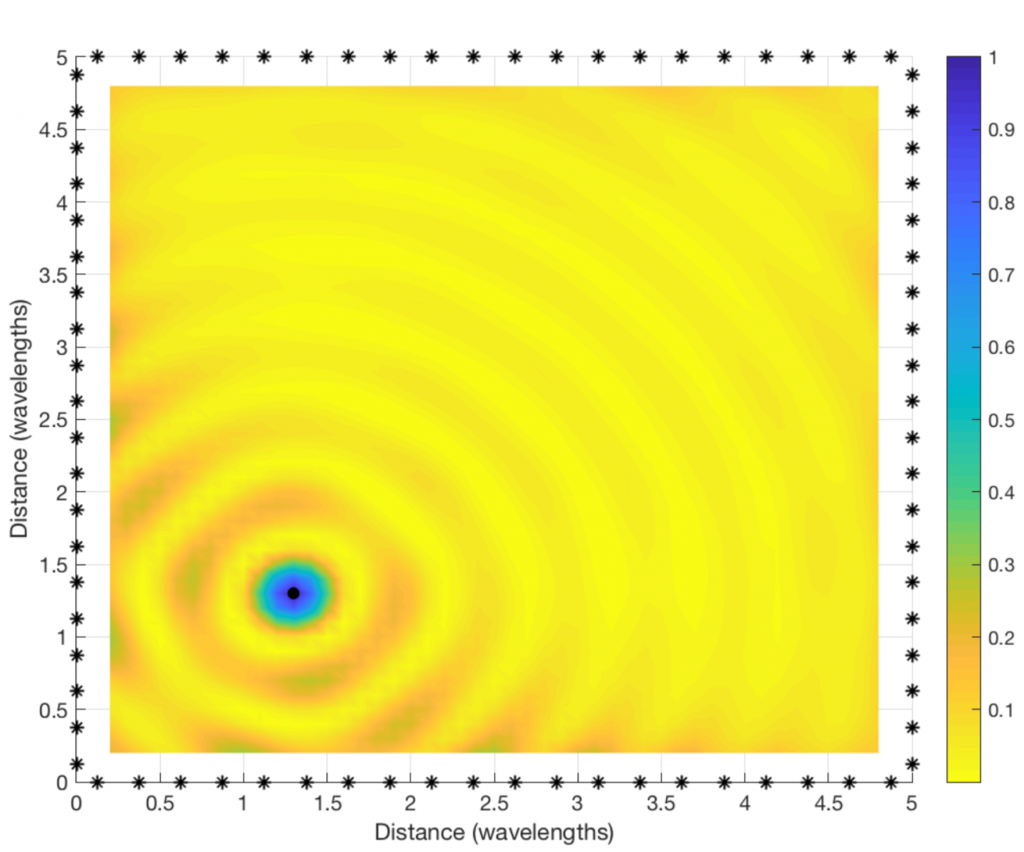
By looking at a two-dimensional version of the figure (see below), we can see that the coherent combination occurs in a circular region that is roughly half a wavelength in diameter. At the carrier frequencies used for cellular networks, this region will only be a few centimeters or millimeters wide. It is almost magical how this distributed array can amplify the signal at such a tiny spatial region! This spatial region is probably what the company Artemis is calling a personal cell (pCell) when marketing their distributed MIMO solution.
If you are into the details, you might wonder why I simulated a square region that is only a few wavelengths wide, and why the antenna spacing is only a quarter of a wavelength. This assumption was only made for illustrative purposes. If the physical antenna locations are fixed but we would reduce the wavelength, the size of the circular region will reduce and the ripples will be more frequent. Hence, we would need to compute the channel gain at many more spatial sample points to produce a smooth plot.
Reproduce the results: The code that was used to produce the plots can be downloaded from my GitHub.
The tedious, time-consuming, and buggy nature of system-level simulations is exacerbated with massive MIMO. This post offers some relieve in the form of analytical expressions for downlink conjugate beamforming [1]. These expressions enable the testing and calibration of simulators—say to determine how many cells are needed to represent an infinitely large network with some desired accuracy. The trick that makes the analysis feasible is to let the shadowing grow strong, yet the ensuing expressions capture very well the behaviors with practical shadowings.
The setting is an infinitely large cellular network where each -antenna base station (BS) serves single-antenna users. The large-scale channel gains include pathloss with exponent and shadowing having log-scale standard deviation , with the gain between the th BS and the th user served by a BS of interest denoted by .With conjugate beamforming and receivers reliant on channel hardening, the signal-to-interference ratio (SIR) at such user is [2]
where is the gain from the serving BS and is the share of that BS’s power allocated to user . Two power allocations can be analyzed:
Uniform: .
SIR-equalizing [3]: , with the proportionality constant ensuring that . This makes . Moreover, as and grow large,
The analysis is conducted for , which makes it valid for arbitrary BS locations.
SIR
For notational compactness, let . Define as the solution to where is the lower incomplete gamma function. For , in particular, . Under a uniform power allocation, the CDF of is available in an explicit form involving the Gauss hypergeometric function (available in MATLAB and Mathematica):
where “” indicates asymptotic () equality, is such that the CDF is continuous, and
Alternatively, the CDF can be obtained by solving (e.g., with Mathematica) a single integral involving the Kummer function :
This latter solution can be modified for the SIR-equalizing power allocation as
Spectral Efficiency
The spectral efficiency of user is with CDF readily characterizable from the expressions given earlier. From , the sum spectral efficiency at the BS of interest can be found as Expressions for the averages and are further available in the form of single integrals.
With a uniform power allocation,
(1)
and . For the special case of , the Kummer function simplifies giving
(2)
With an equal-SIR power allocation
(3)
and .
Application to Relevant Networks
Let us now contrast the analytical expressions (computable instantaneously and exactly, and valid for arbitrary topologies, but asymptotic in the shadowing strength) with some Monte-Carlo simulations (lengthy, noisy, and bug-prone, but for precise shadowing strengths and topologies).
First, we simulate a 500-cell hexagonal lattice with , and . Figs. 1a-1b compare the simulations for – dB with the analysis. The behaviors with these typical outdoor values of are well represented by the analysis and, as it turns out, in rigidly homogeneous networks such as this one is where the gap is largest.
Figure 1: Analysis vs hexagonal network simulations with lognormal shadowing
For a more irregular deployment, let us next consider a network whose BSs are uniformly distributed. BSs (500 on average) are dropped around a central one of interest. For each network snapshot, users are then uniformly dropped until of them are served by the central BS. As before, , and . Figs. 2a-2b compare the simulations for dB with the analysis, and the agreement is now complete. The simulated average spectral efficiency with a uniform power allocation is b/s/Hz/user while (2) gives b/s/Hz/user.
Figure 2: Analysis vs Poisson network simulations with lognornmal shadowing.
The analysis presented in this post is not without limitations, chiefly the absence of noise and pilot contamination. However, as argued in [1], there is a broad operating range (– with very conservative premises) where these effects are rather minor, and the analysis is hence applicable.
The textbook Massive MIMO Networks: Spectral, Energy, and Hardware Efficiency, that I’ve written together with Jakob Hoydis and Luca Sanguinetti, is from now on available for free download from https://massivemimobook.com. If you want a physical copy, you can buy the color-printed hardback edition from now publishers and major online shops, such as Amazon.
You can read more about this book in a previous blog post and also watch this new video, where I talk about the content and motivation behind the writing of the book.
The next generation of cellular networks need to be much more energy-efficient than the current generation, if we should deliver 100-1000 times more data in a cost-efficient and environmentally friendly manner. In this video, I explain the methodology that can be used to design energy efficient 5G networks, and also the key role that Massive MIMO will play.


 -antenna base station (BS) serves
  single-antenna users. The large-scale channel gains include pathloss with exponent
  and shadowing having log-scale standard deviation
  , with the gain between the
  th BS and the
  th user served by a BS of interest denoted by
  .
.
 is the gain from the serving BS and
  is the share of that BS’s power allocated to user
  .
. , with the proportionality constant ensuring that
  . This makes
  . Moreover, as
 , which makes it valid for arbitrary BS locations.
 . Define
  as the solution to
  where
where  is the lower incomplete gamma function. For
  , in particular,
  . Under a uniform power allocation, the CDF of
  is available in an explicit form involving the Gauss hypergeometric function
  (available in MATLAB and Mathematica):
 ” indicates asymptotic (
 ) equality,
  is such that the CDF is continuous, and
 :
:

 with CDF
  readily characterizable from the expressions given earlier. From
  , the sum spectral efficiency at the BS of interest can be found as
  Expressions for the averages
 ![\bar{C} = \mathbb{E} \big[ C_k \big]](http://ma-mimo.ellintech.se/wp-content/ql-cache/quicklatex.com-a887caab28778e8d91a237bcc86a9f3e_l3.png "Rendered by QuickLaTeX.com") and
and ![\bar{C}_{\scriptscriptstyle \Sigma} = \mathbb{E} \! \left[ C_{\scriptscriptstyle \Sigma} \right]](http://ma-mimo.ellintech.se/wp-content/ql-cache/quicklatex.com-865de5351a43ee6f0405ddb531ed84ee_l3.png "Rendered by QuickLaTeX.com") are further available in the form of single integrals.
are further available in the form of single integrals.
 . For the special case of

 ,
,  and
and  –
– dB with the analysis. The behaviors with these typical outdoor values of
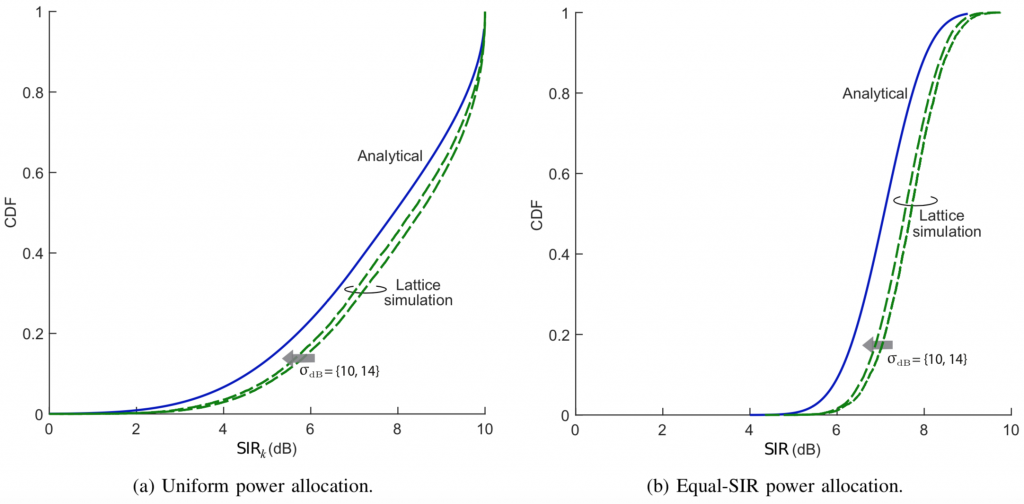
 and
and  . Figs. 2a-2b compare the simulations for
  dB with the analysis, and the agreement is now complete. The simulated average spectral efficiency with a uniform power allocation is
  b/s/Hz/user while (2) gives
  b/s/Hz/user.
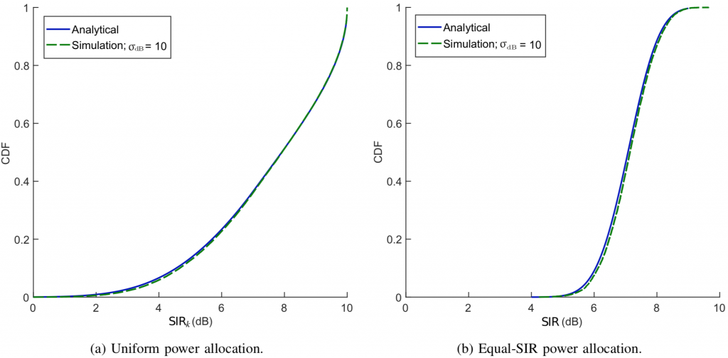
 –
– with very conservative premises) where these effects are rather minor, and the analysis is hence applicable.