
When I went to high school in Sweden, some of my friends stayed up very late at night (due to the time difference) to watch the Super Bowl; the annual championship in the American football league. This game is generally not a big thing in Sweden, but it is huge in America.
This Sunday, the Super Bowl takes place in Atlanta and one million people are expected to come to downtown Atlanta, to either watch the game at the stadium or root for their teams in other ways. Hence, massive flows of images and videos will be posted on social media from people located in a fairly limited area. To prepare for the game, the telecom operators have upgraded their cellular networks and taken the opportunity to market their 5G efforts.
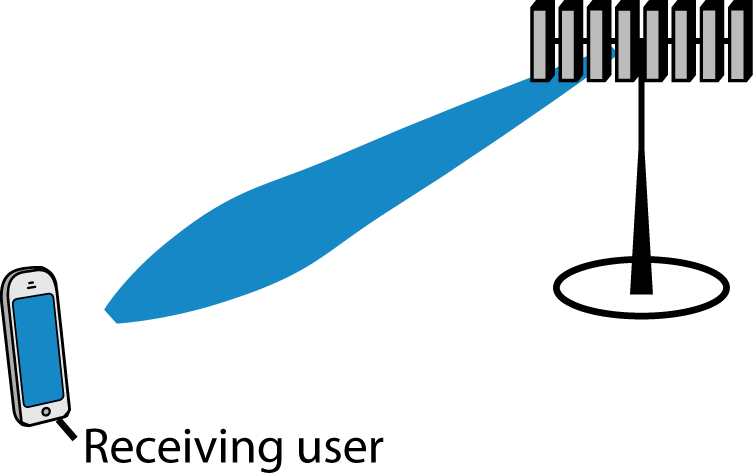
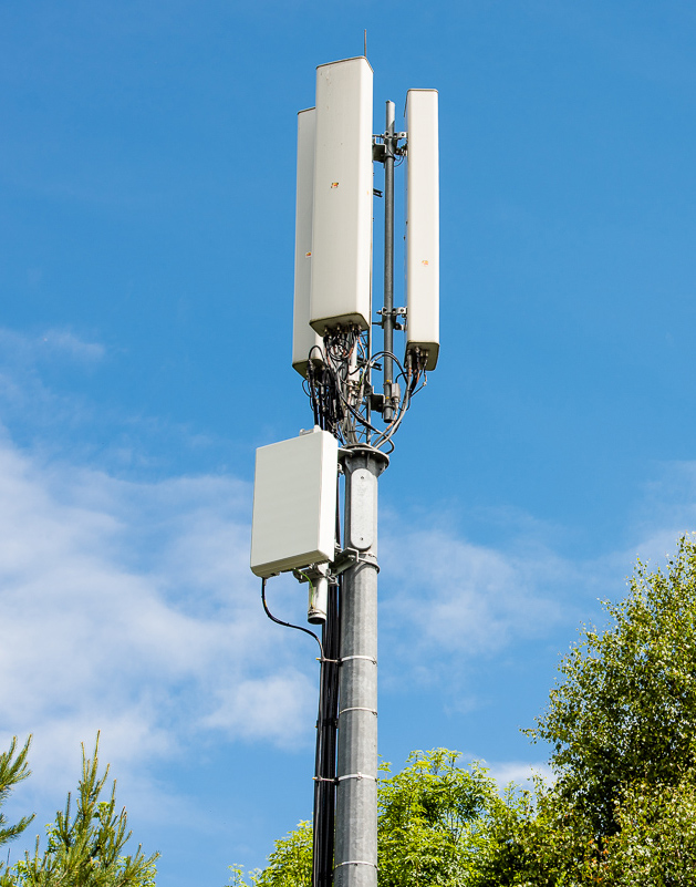
Massive MIMO in the sub-6 GHz band with 64 antennas (and 128 radiating elements) is a key technology to handle the given situation, where huge capacity can be achieved by spatially multiplexing a large number of users in the downtown. Massive MIMO is a “small box with a massive impact” Cyril Mazloum, Network Manager for Sprint in Atlanta, told Hypepotamus. This refers to the fact that the Massive MIMO equipment is, despite the naming, physically smaller than the legacy equipment it replaces. In the following video, Heather Campbell of the Sprint Network Team explains how a ten times higher capacity is achieved in the 2.5 GHz band by their Massive MIMO deployment, which I have also reported about before.
All the major cellular operators have upgraded their networks in preparation for the big game. AT&T has reportedly spent $43 million to deploy 1,500 new antennas. Verizon has installed 30 new macro sites, 300 new small cells, and upgraded the capacity of 150 existing sites. T-Mobile has reportedly boosted its network capacity by eight times. Massive MIMO and 5G are clearly one of the key technologies in all these cases.


 -antenna base station (BS) serves
  single-antenna users. The large-scale channel gains include pathloss with exponent
  and shadowing having log-scale standard deviation
  , with the gain between the
  th BS and the
  th user served by a BS of interest denoted by
  .
.
 is the gain from the serving BS and
  is the share of that BS’s power allocated to user
  .
. , with the proportionality constant ensuring that
  . This makes
  . Moreover, as
 , which makes it valid for arbitrary BS locations.
 . Define
  as the solution to
  where
where  is the lower incomplete gamma function. For
  , in particular,
  . Under a uniform power allocation, the CDF of
  is available in an explicit form involving the Gauss hypergeometric function
  (available in MATLAB and Mathematica):
 ” indicates asymptotic (
 ) equality,
  is such that the CDF is continuous, and
 :
:

 with CDF
  readily characterizable from the expressions given earlier. From
  , the sum spectral efficiency at the BS of interest can be found as
  Expressions for the averages
 ![\bar{C} = \mathbb{E} \big[ C_k \big]](http://ma-mimo.ellintech.se/wp-content/ql-cache/quicklatex.com-a887caab28778e8d91a237bcc86a9f3e_l3.png "Rendered by QuickLaTeX.com") and
and ![\bar{C}_{\scriptscriptstyle \Sigma} = \mathbb{E} \! \left[ C_{\scriptscriptstyle \Sigma} \right]](http://ma-mimo.ellintech.se/wp-content/ql-cache/quicklatex.com-865de5351a43ee6f0405ddb531ed84ee_l3.png "Rendered by QuickLaTeX.com") are further available in the form of single integrals.
are further available in the form of single integrals.
 . For the special case of

 ,
,  and
and  –
– dB with the analysis. The behaviors with these typical outdoor values of
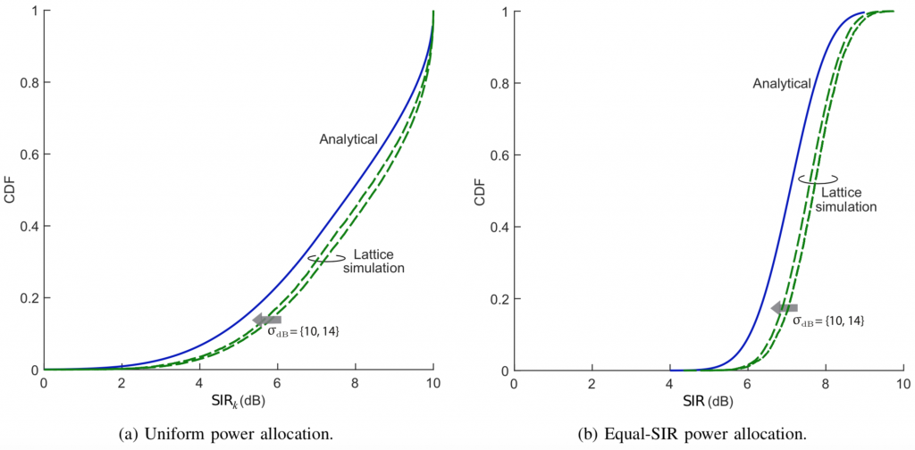
 and
and  . Figs. 2a-2b compare the simulations for
  dB with the analysis, and the agreement is now complete. The simulated average spectral efficiency with a uniform power allocation is
  b/s/Hz/user while (2) gives
  b/s/Hz/user.
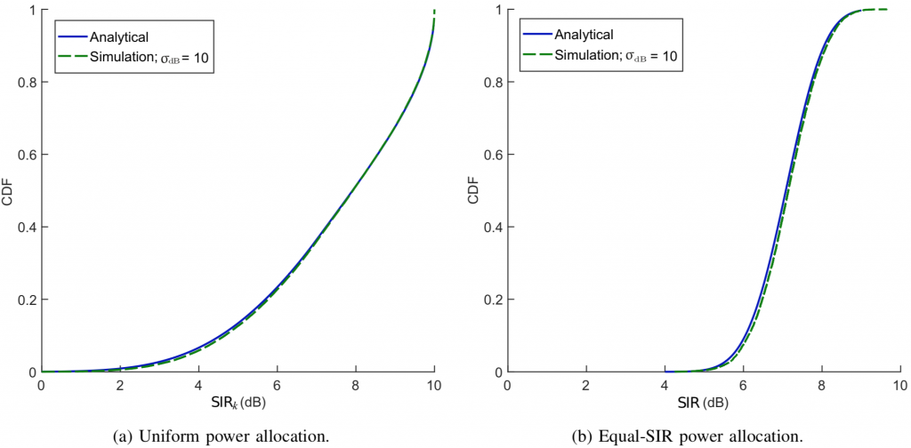
 –
– with very conservative premises) where these effects are rather minor, and the analysis is hence applicable.