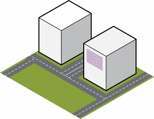
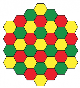
Cellular Multi-User MIMO: A Technology Whose Time has Come

Both the number of devices with wireless connection and the traffic that they generate have steadily grown since the early days of cellular communications. This continuously calls for improvements in the area capacity [bit/s/km2] of the networks. The use of adaptive antenna arrays was identified as a potential capacity-improving technology in the mid-eighties. An early uplink paper was “Optimum combining for indoor radio systems with multiple users” from 1987 by J. Winters at Bell Labs. An early downlink paper was “The performance enhancement of multibeam adaptive base-station antennas for cellular land mobile radio systems” by S. C. Swales et al. from 1990.

The multi-user MIMO concept, then called space-division multiple access (SDMA), was picked up by the industry in the nineties. For example, Ericsson made field-trials with antenna arrays in GSM systems, which were reported in “Adaptive antennas for GSM and TDMA systems” from 1999. ArrayComm filed an SDMA patent in 1991 and made trials in the nineties. In cooperation with the manufacturer Kyocera, this resulted in commercial deployment of SDMA as an overlay to the TDD-based Personal Handy-phone System (PHS).

Trial with a 12-element circular array by ArrayComm, in the late nineties.


Given this history, why isn’t multi-user MIMO a key ingredient in current cellular networks? I think there are several answers to this question:

  1. Most cellular networks use FDD spectrum. To acquire the downlink channels, the SDMA research first focused on angle-of-arrival estimation and later on beamforming codebooks. The cellular propagation environments turned out to be far more complicated than such system concepts easily can handle.
  2. The breakthroughs in information theory for multi-user MIMO happened in the early 2000s, thus there was no theoretical framework that the industry could use in the nineties to evaluate and optimize their multiple antenna concepts.
  3. In practice, it has been far easier to increase the area capacity by deploying more base stations and using more spectrum, rather than developing more advanced base station hardware. In current networks, there is typically zero, one or two users per cell active at a time, and then there is little need for multi-user MIMO.

Why is multi-user MIMO considered a key 5G technology? Basically because the three issues described above have now changed substantially. There is a renewed interest in TDD, with successful cellular deployments in Asia and WiFi being used everywhere. Massive MIMO is the refined form of multi-user MIMO, where the TDD operation enables channel estimation in any propagation environment, the many antennas allow for low-complexity signal processing, and the scalable protocols are suitable for large-scale deployments. The technology can nowadays be implemented using power-efficient off-the-shelf radio-frequency transceivers, as demonstrated by testbeds. Massive MIMO builds upon a solid ground of information theory, which shows how to communicate efficiently under practical impairments such as interference and imperfect channel knowledge.

Maybe most importantly, spatial multiplexing is needed to manage the future data traffic growth. This is because deploying many more base stations or obtaining much more spectrum are not viable options if we want to maintain network coverage—small cells at the street-level are easily shadowed by buildings and mm-wave frequency signals do not propagate well though walls. In 5G networks, a typical cellular base station might have tens of active users at a time, which is a sufficient number to benefit from the great spectral efficiency offered by Massive MIMO.

Definition of Massive MIMO

What is Massive MIMO?  The term has been used for many different systems and the only common denominator seems to be a multi-user MIMO system with everything between 10 to infinitely many antennas.  In the book [1], the authors give the following definition:

“Massive MIMO is a useful and scalable version of Multiuser MIMO.  There are three fundamental distinctions between Massive MIMO and conventional Multiuser MIMO. First, only the base station learns G. Second, M is typically much larger than K, although this does not have to be the case. Third, simple linear signal processing is used both on the uplink and on the downlink. These features render Massive MIMO scalable with respect to the number of base station antennas, M.”

(Note: M is the number of antennas, K is the number of users, and G denotes the channel matrix).

In [2], we find another definition:

“Massive MIMO is a multi-user MIMO system with M antennas and K users per BS. The system is characterized by M ≫ K and operates in TDD mode using linear uplink and downlink processing.”

Both are nice general definitions that cover most systems that commonly are called “Massive MIMO”.  However, their generality also makes them vague and they fail to pinpoint the essence of Massive MIMO.  Here, is my take on a slightly more precise definition:

“Massive MIMO is a multi-user MIMO system that (1) serves multiple users through spatial multiplexing over a channel with favorable propagation in time-division duplex and (2) relies on channel reciprocity and uplink pilots to obtain channel state information.”

Now, you might ask: So what is then “favorable propagation”?  We need a second definition:

“The propagation is said to be favorable when users are mutually orthogonal in some practical sense.”

Again you ask: in what practical sense?  If h∈ℂᴹ is the channel vector to one user and g∈ℂᴹ the channel vector to another, the users are said to be orthogonal if hg = 0.  Unfortunately, this is never true in a real system.  It can be practically true, however, if we say that users are practically orthogonal when hg/(‖h‖‖g‖) has mean zero and a variance that is much smaller than one.

There we go: a more-or-less rigorous definition of Massive MIMO.  Note that this definition does not require the number of users to be small in any sense.  So, to the big question: How many antennas does a base station need to be “massive”? The answer is given for the i.i.d. Rayleigh fading channel in the following curve that shows how the users’ channels become practically orthogonal as the number of antennas is increased.

Variance
Massive MIMO base stations have more than 100 antennas


  1. [1] T. L. Marzetta, E. G. Larsson, H. Yang, N. Q. Ngo. Fundamentals of Massive MIMO. Cambridge University Press, 2016.
  2. [2] T. V. Chien, E. Björnson, “Massive MIMO Communications,” in 5G Mobile Communications, W. Xiang et al. (eds.), pp. 77-116, Springer, 2017.

How Many Antennas are Useful?

One question tends to reoccur: How many antennas can a Massive MIMO base station usefully deploy? Current thinking for macro-cellular is that 100-200 antennas would be suitable. Will we in the future see a lot more, thousands or so?

In that application, I don’t think so. Here is why.

What ultimately limits Massive MIMO is mobility: no more than half of the coherence time-bandwidth product should be occupied by pilot transmission activities. (This is the “half and half rule”.) In macro-cellular at 3 GHz, with highway mobility we may have on the order of 200 kHz x 1 millisecond coherence; that is 200 samples. With pilot reuse of 3 (that practically does away with pilot contamination), we could, then ultimately learn the channel to some 30 simultaneously served terminals – assuming mutually orthogonal pilots. Once the number of base station antennas M reaches beyond twice this number, with some margin – say M=100, the spectral efficiency grows logarithmically with M. That means, even doubling M yields only a 3dB effective SINR increase, that is a single extra bit per second/Hz per terminal. Beyond M=100 or M=200, it may not be worth it. Multiple antennas are only truly useful if they are used to multiplex, and mobility limits the amount of multiplexing we can perform.

So why not quadruple the number of antennas for additional coverage? May not be worth it either. Going from M=200 to M=2000 gives 10 dB – that pays for a 75% range extension, or, alternatively, a tenth of the losses incurred by an energy-saving coated window glass.

In stationary environments, the story is different – a topic that we will be returning to.

How distant into the future?

Are There Any Massive MIMO Books?

9781107175570_200x_fundamentals-of-massive-mimoI regularly get the question “are there any Massive MIMO books?”. So far my answer has always been “no”, but now I can finally give a positive answer.

My colleagues Erik G. Larsson and Hien Quoc Ngo have written a book entitled “Fundamentals of Massive MIMO” together with Thomas L. Marzetta and Hong Yang at Bell Labs, Nokia. The book is published this October/November by Cambridge University Press.

I have read the book and I think it serves as an excellent introduction to the topic. The text is suitable for graduate students, practicing engineers, professors, and doctoral students who would like to learn the basic Massive MIMO concept, results and properties. It also provides a clean introduction to the theoretical tools that are suitable for analyzing the Massive MIMO performance.

I personally intend to use this book as course material for a Master level course on Multiple-antenna communications next year. I recommend other teachers to also consider this possibility!

A preview of the book can be found on Google Books:

Update: Since November 2017, there is another book: “Massive MIMO Networks: Spectral, Energy, and Hardware Efficiency“.

How Much does Massive MIMO Improve the Spectral Efficiency?

It is often claimed in the academic literature that Massive MIMO can greatly improve the spectral efficiency. What does it mean, qualitatively and quantitatively? This is what I will try to explain.

With spectral efficiency, we usually mean the sum spectral efficiency of the transmissions in a cell of a cellular network. It is measured in bit/s/Hz. If you multiply it with the bandwidth, you will get the cell throughput measured in bit/s. Since the bandwidth is a scarce resource, particularly at the frequencies below 5 GHz that are suitable for network coverage, it is highly desirable to improve the cell throughput by increasing the spectral efficiency rather than increasing the bandwidth.

A great way to improve the spectral efficiency is to simultaneously serve many user terminals in the cell, over the same bandwidth, by means of space division multiple access. This is where Massive MIMO is king. There is no doubt that this technology can improve the spectral efficiency. The question is rather “how much?”

Earlier this year, the joint experimental effort by the universities in Bristol and Lund demonstrated an impressive spectral efficiency of 145.6 bit/s/Hz, over a 20 MHz bandwidth in the 3.5 GHz band. The experiment was carried out in a single-cell indoor environment. Their huge spectral efficiency can be compared with 3 bit/s/Hz, which is the IMT Advanced requirement for 4G. The remarkable Massive MIMO gain was achieved by spatial multiplexing of data signals to 22 users using 256-QAM. The raw spectral efficiency is 176 bit/s/Hz, but 17% was lost for practical reasons. You can read more about this measurement campaign here:

http://www.bristol.ac.uk/news/2016/may/5g-wireless-spectrum-efficiency.html

256-QAM is generally not an option in cellular networks, due to the inter-cell interference and unfavorable cell edge conditions. Numerical simulations can, however, predict the practically achievable spectral efficiency. The figure below shows the uplink spectral efficiency for a base station with 200 antennas that serves a varying number of users. Interference from many tiers of neighboring cells is considered. Zero-forcing detection, pilot-based channel estimation, and power control that gives every user 0 dB SNR are assumed. Different curves are shown for different values of τc, which is the number of symbols per channel coherence interval. The curves have several peaks, since the results are optimized over different pilot reuse factors.

Spectral efficiency
Uplink spectral efficiency in a cellular network with 200 base station antennas.

From this simulation figure we observe that the spectral efficiency grows linearly with the number of users, for the first 30-40 users. For larger user numbers, the spectral efficiency saturates due to interference and limited channel coherence. The top value of each curve is in the range from 60 to 110 bit/s/Hz, which are remarkable improvements over the 3 bit/s/Hz of IMT Advanced.

In conclusion, 20x-40x improvements in spectral efficiency over IMT Advanced are what to expect from Massive MIMO.

Are 1-bit ADCs Sufficient?

A series of recent papers,

suggest the use of 1-bit ADCs in Massive MIMO base station receivers. Important studies of a concept, that offers great potential for cost saving and simplification of transceiver hardware.

One-bit ADCs
One-bit ADCs quantize the sign of the real and imaginary part of the complex baseband signal.


Granted, much lower resolution will be sufficient in Massive MIMO than in conventional MIMO, but will one bit be sufficient? These papers indicate that the price to pay is not insignificant: the number of antennas may have to be doubled in some cases. Also, while the use of symbol-sampled models as in these studies may give correct order-of-magnitude estimates of capacity, much future work appears to remain to understand the effects of digital channelization/prefiltering and sampling rate conversion if 1-bit frontends are going to be used.

Massive MIMO in Mobile Environments

An impressive experiment, recently reported by colleagues at Univ. of Lund and Univ. of Bristol, shows TDD (reciprocity-based) Massive MIMO multiplexing to mobile terminals:

The interesting part starts at 2:48, with the terminals onboard cars. While it has been contested whether Massive MIMO can work in mobility (because of channel aging) this experiment confirms that it does — as predicted by theory for a long time. In fact, at 3.7 GHz carrier and with a slot length of 0.5 ms, the maximum permitted mobility (assuming a two-ray model with Nyquist sampling, and a factor-of-two design margin) is over 140 km/h. So the experiment is probably still not close to the physical limits.

News – commentary – mythbusting