The good side of the social distancing that is currently taking place is that I have spent more time recording video material than usual. For example, I was supposed to give a tutorial entitled “Signal Processing for MIMO Communications Beyond 5G” at ICASSP 2020 in Barcelona in the beginning of May. This conference has now turned into an online event with free registration. Hence, anyone can attend the tutorial that I am giving together with Jiayi Zhang from Beijing Jiaotong University. We have prerecorded the presentations, which will be broadcasted to the conference attendees on May 4, but will be available for live discussions in between each video segment.
As a teaser for this tutorial, I have uploaded the 30 minute introduction to YouTube:
In this video, I explain what Massive MIMO is, what role it plays in 5G, why there will be a large gap between the theoretical performance and what is achieved in practice, and what might come next. In particular, I explain my philosophy regarding 6G research.
The remaining 2.5 hours of the tutorial will only be available from ICASSP. I hope to meet you online on May 4!
Line-of-sight channels normally contain many propagation paths, whereof one is the direct path and the others are paths were the signals are scattered on different objects. The interaction between these paths lead to fading phenomena, which is often modeled statistically using Rician fading (sometimes written as Ricean fading). The main assumption is that the complex-valued channel coefficient in the complex baseband can be divided into two parts:
where is the magnitude of the direct path between the transmitter and receiver and is the corresponding phase shift. The second part, , represents all the scattered paths. This part is separated from the direct path since it consists of many paths, each being of roughly the same strength but substantially weaker than the direct path. It is modeled by Rayleigh fading, which implies . The complex Gaussian distribution is motivated by the central limit theorem, which says that the sum of many independent and identically distributed random variables is approximately Gaussian.
Under these assumptions, the magnitude of the channel coefficient is Rice/Rician distributed, which is why it is called Rician fading. More precisely, , which depends on the magnitude and the variance of the scattering.
Interestingly, the distribution does not depend on the phase , because the magnitude removes phases and and are equally distributed. Hence, it is common to omit in the performance analysis of Rician fading channels. As long as the channel is perfectly known at the receiver, it will not make any difference when quantifying the SNR or capacity.
The common misunderstanding
We cannot neglect the phase when analyzing practical systems where the receiver needs to estimate the channel. The value of varies at the same pace as , and for exactly the same reason: The transmitter or receiver moves, which induces small phase shifts in every path. Since contains a large number of paths with approximately the same magnitude but random phases, the sum of the many terms with random phases give rise to the Gaussian distribution. The phase-shift of the direct path must be treated separately since this path is substantially stronger.
Unfortunately, my experience is that the vast majority of paper on Rician fading channels ignores this fact by simply treating as a deterministic constant that is perfectly known at the receiver. I have done this myself in several papers, including this one from 2010 that has received 200+ citations. Unfortunately, the results obtained with that simplified model are practically questionable. If we don’t know in advance, how can we know ? At best, the results obtained with a perfectly known can be interpreted as an upper bound on what is practically achievable.
We analyzed the importance of correctly modeled random phases in a recent paper on cell-free massive MIMO. We compared the performance when using an ideal phase-aware MMSE estimator and a phase-unaware LMMSE estimator. The spectral efficiency loss due to a lack of knowing ranges from 2% to 50% in different simulations, depending on the pilot length and interference situation. Hence, there are cases where it is very important to know the phase correctly.
A defining factor for the early Massive MIMO literature is the study of communication systems where the number of base station antennas goes to infinity. Marzetta’s original paper considered this asymptotic regime from the outset. Many other papers derived rate expressions for a finite value, and then studied their behavior as . In these papers, the signal-to-noise ratio (SNR) grows linearly with , and the rate grows towards infinity as (except when pilot contamination is a limiting factor).
I have carried out such asymptotic analysis myself, but there is one issue that has been disturbing me for a while: The SNR cannot grow without bound in practice because we can never receive more power than what was transmitted from the base station. It doesn’t matter how many transmit antennas that are used or how razor-sharp the beams become, the law of conservation of energy must be respected. So where is the error in the analysis?
The problem is not that implies the use of infinitely large arrays. If we accept that the universe is infinite, it is plausible to create an -antenna planar array for any value of , for example, using a grid. Such an array is illustrated in Figure 1.
Figure 1: A planar array with 9 x 9 antennas are used to communicate with a user device.
The actual issue is how the channel gains (pathlosses) between the antennas and the user are modeled. We are used to considering channel models based on far-field approximations, where the channel gain is the same for all antennas (when averaging over small-scale fading). However, as the size of the array grows, the approximate far-field models become inaccurate. Instead, one needs to model the following phenomena that appear in the near-field:
The propagation distance is different between each base station antenna and the user.
The effective antenna areas vary in the array, even if the physical areas are equal, since the antennas are observed from different angles.
The polarization losses vary between the antennas, because of the different angles from the antennas to the user.
It might seem complicated to take these phenomena into account, but the following paper shows how to compute the channel gain exactly when the user is centered in front of the array. I generalized this formula to non-centered users in a new paper. We utilized the new result to study the asymptotic behaviors of Massive MIMO and also intelligent reflecting surfaces. It turned out that all the three aforementioned phenomena are important to get accurate asymptotic results. When transmitting from an isotropic antenna to a planar Massive MIMO array, the total channel gain converges to 1/3 and instead of going to infinity. The remaining 2/3 of the transmit power is lost due to polarization mismatch or radiation into the opposite direction of the array. If any of the first two phenomena are ignored, the channel gain will grow unboundedly as , which is physically impossible. If the last one is ignored, the asymptotic channel gain is overestimated by 50%, so this is the least critical factor.
Although the exact channel model can be used to accurately predict the asymptotic SNR behavior, my experience from studying this topic is that the far-field approximations are accurate in most cases of practical interest. It is first when the propagation distance is shorter than the side length of the array that the near-field phenomena are critically important. In other words, the scaling laws that have been obtained in the Massive MIMO literature are usually applicable in practice, even if they break down asymptotically.
The hype around machine learning, particularly deep learning, has spread over the world. It is not only affecting engineers but also philosophers and government agencies, which try to predict what implications machine learning will have on our society.
When the initial excitement has subsided, I think machine learning will be an important tool that many engineers will find useful, alongside more classical tools such as optimization theory and Fourier analysis. I have spent the last two years thinking about what role deep learning can have in the field of communications. This field is rather different from other areas where deep learning has been successful: We deal with man-made systems that have designed based on rigorous theory to operate close to the fundamental performance limits, for example, the Shannon capacity. Hence, at first sight, there seems to be little room for improvement.
I have nevertheless identified two main applications of supervised deep learning in the physical layer of communication systems: 1) algorithmic approximation and 2) function inversion.
In the video, I’m exemplifying the applications through two recent papers where we applied deep learning to improve Massive MIMO systems. Here are links to those papers:
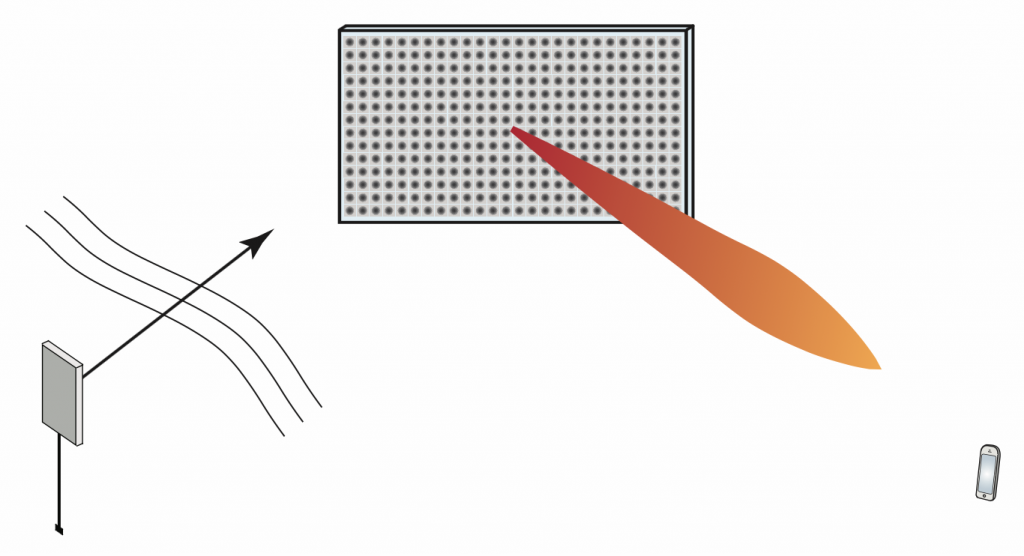
Emerging intelligent reflecting surface (IRS) technology, also known under the names “reconfigurable intelligent surface” and “software-controlled metasurface”, is sometimes marketed as an enabling technology for 6G. How do they work, what are their use cases and how much will they improve wireless access performance at large?
The physical principle of an IRS is that the surface is composed of atoms, each of which acts as an “intelligent” scatterer: a small antenna that receives and re-radiates without amplification, but with a controllable phase-shift. Typically, an atom is implemented as a small patch antenna terminated with an adjustable impedance. Assuming the phase shifts are properly adjusted, the scattered wavefronts can be made to add up constructively at the receiver. If coupling between the atoms is neglected, the analysis of an IRS essentially entails (i) finding the Green’s function of the source (a sum of spherical waves if close, or a plane wave if far away), (ii) computing the impinging field at each atom, (iii) integrating this field over the surface of each atom to find a current density, (iv) computing the radiated field from each atom using physical-optics approximation, and (v) applying the superposition principle to find the field at the receiver. If the atoms are electrically small, one can approximate the re-radiated field by pretending the atoms are point sources and then the received “signal” is basically a superposition of phase-shifted (as ), amplitude-scaled (as ) source signals.
A point worth re-iterating is that an atom is a scatterer, not a “mirror”. A more subtle point is that the entire IRS as such, consisting of a collection of scatterers, is itself also a scatterer, not a mirror. “Mirrors” exist only in textbooks, when a plane wave is impinging onto an infinitely large conducting plate (none of which exist in practice). Irrespective of how the IRS is constructed, if it is viewed from far enough away, its radiated field will have a beamwidth that is inversely proportional to its size measured in wavelengths.
Two different operating regimes of IRSs can be distinguished:
1. Both transmitter and receiver are in the far-field of the surface. Then the waves seen at the surface can be approximated as planar; the phase differential from the surface center to its edge is less than a few degrees, say. In this case the phase shifts applied to each atom should be linear in the surface coordinate. The foreseen use case would be to improve coverage, or provide an extra path to improve the rank of a point-to-point MIMO channel. Unfortunately in this case the transmitter-IRS-path loss scales very unfavorably, as where is the number of meta-atoms in the surface, and the reason is that again, the IRS itself acts as a (large) scatterer, not a “mirror”. Therefore the IRS has to be quite large before it becomes competitive with a standard single-antenna decode-and-forward relay, a simple, well understood technology that can be implemented using already widely available components, at small power consumption and with a small form factor. (In addition, full-duplex technology is emerging and may eventually be combined with relaying, or even massive MIMO relaying.)
2. At least one of the transmitter and the receiver is in the surface near-field. Here the plane-wave approximation is no longer valid. The IRS can then either be sub-optimally configured to act as a “mirror”, in which case the phase shifts vary linearly as function of the surface coordinate. Alternatively, it can be configured to act as a “lens”, with optimized phase-shifts, which is typically better. As shown for example in this paper, in the near-field case the path loss scales more favorably than in the far-field case. The use cases for the near-field case are less obvious, but one can think of perhaps indoor environments with users close to the walls and every wall covered by an IRS. Another potential use case that I learned about recently is to use the IRS as a MIMO transmitter: a single-antenna transmitter near an IRS can be jointly configured to act as a MIMO beamforming array.
So how useful will IRS technology be in 6G? The question seems open. Indoor coverage in niche scenarios, but isn’t this an already solved problem? Outdoor coverage improvement, but then (cell-free) massive MIMO seems to be a much better option? Building MIMO transmitters from a single-antenna seems exciting, but is it better than using conventional RF? Perhaps it is for the Terahertz bands, where implementation of coherent MIMO may prove truly challenging, that IRS technology will be most beneficial.
A final point is that nothing requires the atoms in an IRS to be located adjacently to one another, or even to form a surface! But they are probably easier to coordinate if they are in more or less the same place.
By deploying many distributed antennas instead of a few multi-antenna base stations, a more uniform communication performance can be achieved over a coverage area. The peak rates might go down but there is a much higher chance of getting a decent rate with 95% probability. This is the main motivation behind Cell-free Massive MIMO, which is the new name for Network MIMO with a large number of antennas (many more than the number of users). The key difference from conventional ultra-dense networks is that the distributed antennas are cooperating to transmit phase-coherently in the downlink and process the received uplink signals coherently. One promising way to deploy these systems is by using radio stripes.
The first papers on Cell-free Massive MIMO assumed that all antennas have access to the downlink data of all users and take part in the uplink signal detection of all users. This is both impractical and unnecessary in a large network, where each user is only physically close to a subset of the antennas. Hence, it makes practical sense that only those antennas that can reach the user with a signal power that is non-negligible compared to the thermal noise should transmit to that user and participate in the detection of its uplink data.
I designed a framework for this 10 years ago, which I called “dynamic cooperation clusters” (DCC) and it can be readily applied to Cell-free Massive MIMO. The main idea was that every user selects which antennas should serve it in a user-centric manner, which means that any antenna subset can be selected. This stands in contrast to the conventional network-centric approach (which dominated the 4G CoMP literature) where only certain predefined disjoint groups of antennas are allowed to cooperate.
Although the DCC framework is a perfect fit for Cell-free Massive MIMO, the performance analysis that we did 10 years ago was admittedly simplified compared to what is possible with the latest methodology. We considered TDD systems that utilize reciprocity but assumed slowly fading channels that can be estimated without error, thereby avoiding pilot contamination and the computation of ergodic rates. To provide a bridge to the past, we wrote the paper “Scalable Cell-Free Massive MIMO Systems” which revisits the DCC framework in the context of Cell-free Massive MIMO, using the latest analytical methods from the Massive MIMO literature.
Most importantly, the new paper provides an intuitive way to select the user-centric cooperation clusters based on the uplink pilot transmissions. When a user connects to the network, we suggest that the antenna with the best channel condition is given the responsibility to guarantee the user service. The user is assigned to the pilot that is least affected by pilot contamination in that particular region. Moreover, all antennas serve as many users as there are pilots; at most one user per pilot to limit the negative effect of pilot contamination. Under these assumptions, we show that the users get nearly the same rates as if all the antennas serve all users, but with greatly reduced complexity and fronthaul requirements. In conclusion, scalable and well-performing implementations of Cell-free Massive MIMO are possible!
I have recorded a popular science video that explains how a cell-free network architecture can provide major performance improvements over 5G cellular networks, and why radio stripes is a promising way to implement it:
If you want more technical details, I recommend our recent survey paper “Ubiquitous Cell-Free Massive MIMO Communications“. One of the authors, Dr. Hien Quoc Ngo at Queen’s University Belfast, has created a blog about Cell-free Massive MIMO. In particular, it contains a list of papers on the topic and links to the programming code of some of them.

 in the complex baseband can be divided into two parts:
 is the magnitude of the direct path between the transmitter and receiver and
 ![\theta \in [0,2\pi]](http://ma-mimo.ellintech.se/wp-content/ql-cache/quicklatex.com-e70126963911574a22ab8afc7da04ca9_l3.png "Rendered by QuickLaTeX.com") is the corresponding phase shift. The second part,
is the corresponding phase shift. The second part,  , represents all the scattered paths. This part is separated from the direct path since it consists of many paths, each being of roughly the same strength but substantially weaker than the direct path. It is modeled by Rayleigh fading, which implies
  . The complex Gaussian distribution is motivated by the
  of the channel coefficient is
  , which depends on the magnitude
  and the variance
  of the scattering.
 , because the magnitude removes phases and
  are equally distributed. Hence, it is common to omit
  as a deterministic constant that is perfectly known at the receiver. I have done this myself in several papers, including
  goes to infinity. Marzetta’s
  . In these papers, the signal-to-noise ratio (SNR) grows linearly with
  (except when pilot contamination
  grid. Such an array is illustrated in Figure 1.
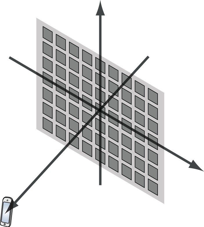
 atoms, each of which acts as an “intelligent” scatterer: a small antenna that receives and re-radiates without amplification, but with a controllable phase-shift. Typically, an atom is implemented as a small patch antenna terminated with an adjustable impedance. Assuming the phase shifts are properly adjusted, the
  ), amplitude-scaled (as
  ) source signals.
 where
where