The channel between a single-antenna user and an  -antenna base station can be represented by an -dimensional channel vector. The canonical channel model in the Massive MIMO literature is independent and identically distributed (i.i.d.) Rayleigh fading, in which the vector is a circularly symmetric complex Gaussian random variable with a scaled identity matrix as correlation/covariance matrix:
  , where
  is the variance.
With i.i.d. Rayleigh fading, the channel gain  has an Erlang
 -distribution (this is a scaled
  distribution) and the channel direction
  is uniformly distributed over the unit sphere in
  . The channel gain and the channel direction are also independent random variables, which is why this is a spatially uncorrelated channel model.
One of the key benefits of i.i.d. Rayleigh fading is that one can compute closed-form rate expressions, at least when using maximum ratio or zero-forcing processing; see Fundamentals of Massive MIMO for details. These expressions have an intuitive interpretation, but should be treated with care because practical channels are not spatially uncorrelated. Firstly, due to the propagation environment, the channel vector is more probable to point in some directions than in others. Secondly, the antennas have spatially dependent antenna patterns. Both factors contribute to the fact that spatial channel correlation always appears in practice.
One of the basic properties of spatial channel correlation is that the base station array receives different average signal power from different spatial directions. This is illustrated in Figure 1 below for a uniform linear array with 100 antennas, where the angle of arrival is measured from the boresight of the array.
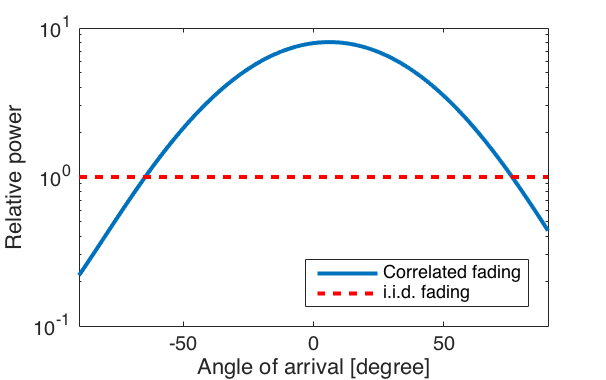
As seen from Figure 1, with i.i.d. Rayleigh fading the average received power is equally large from all directions, while with spatially correlated fading it varies depending on in which direction the base station applies its receive beamforming. Note that this is a numerical example that was generated by letting the signal come from four scattering clusters located in different angular directions. Channel measurements from Lund University (see Figure 4 in this paper) show how the spatial correlation behaves in practical scenarios.
Correlated Rayleigh fading is a tractable way to model a spatially correlation channel vector:  , where the covariance matrix
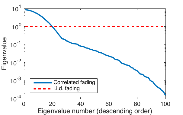
  is also the correlation matrix. It is only when is a scaled identity matrix that we have spatially uncorrelated fading. The eigenvalue distribution determines how strongly spatially correlated the channel is. If all eigenvalues are identical, then is a scaled identity matrix and there is no spatial correlation. If there are a few strong eigenvalues that contain most of the power, then there is very strong spatial correlation and the channel vector is very likely to be (approximately) spanned by the corresponding eigenvectors. This is illustrated in Figure 2 below, for the same scenario as in the previous figure. In the considered correlated fading case, there are 20 eigenvalues that are larger than in the i.i.d. fading case. These eigenvalues contain 94% of the power, while the next 20 eigenvalues contain 5% and the smallest 60 eigenvalues only contain 1%. Hence, most of the power is concentrated to a subspace of dimension
  . The fraction of strong eigenvalues is related to the fraction of the angular interval from which strong signals are received. This relation can be made explicit in special cases.
One example of spatially correlated fading is when the correlation matrix has equal diagonal elements and non-zero off-diagonal elements, which describe the correlation between the channel coefficients of different antennas. This is a reasonable model when deploying a compact base station array in tower. Another example is a diagonal correlation matrix with different diagonal elements. This is a reasonable model when deploying distributed antennas, as in the case of cell-free Massive MIMO.
Finally, a more general channel model is correlated Rician fading:  , where the mean value
  represents the deterministic line-of-sight channel and the covariance matrix determines the properties of the fading. The correlation matrix
  can still be used to determine the spatial correlation of the received signal power. However, from a system performance perspective, the fraction
  between the power of the line-of-sight path and the scattered paths can have a large impact on the performance as well. A nearly deterministic channel with a large
  -factor provide more reliable communication, in particular since under correlated fading it is only the large eigenvalues of that contributes to the channel hardening (which otherwise provides reliability in Massive MIMO).

 :
:

 and
and  denote the number of cells and UEs per cell,
  is the estimated channel matrix from the UEs in cell
  and
and  are the covariance matrices of the channel and the channel estimation errors of UE
  in cell
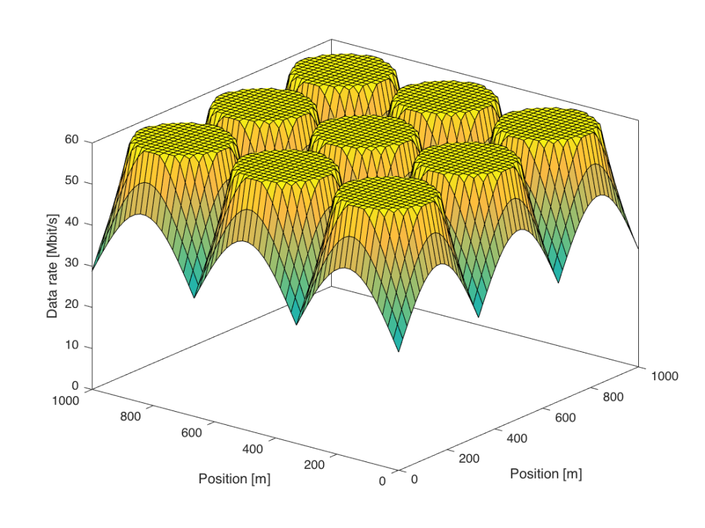
  , respectively. While M-MMSE combining uses estimates of the channels from all UEs in all cells, the simpler S-MMSE combining uses only channel estimates from the UEs in the own cell. Importantly, we show that Massive MIMO with M-MMSE combining has unlimited capacity while Massive MIMO with S-MMSE combining has not! This behavior is shown in the following figure:
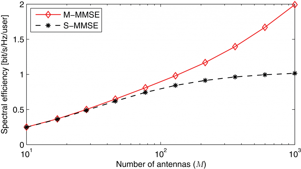
 (…) to further
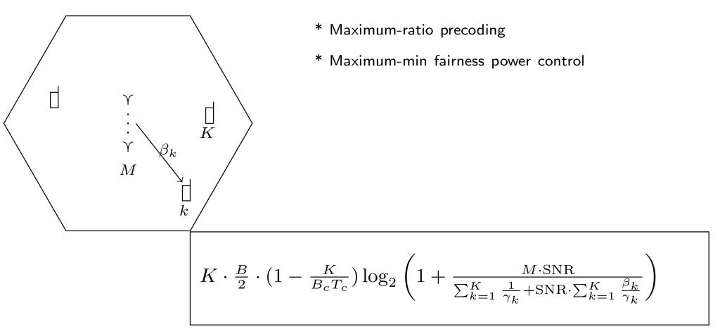
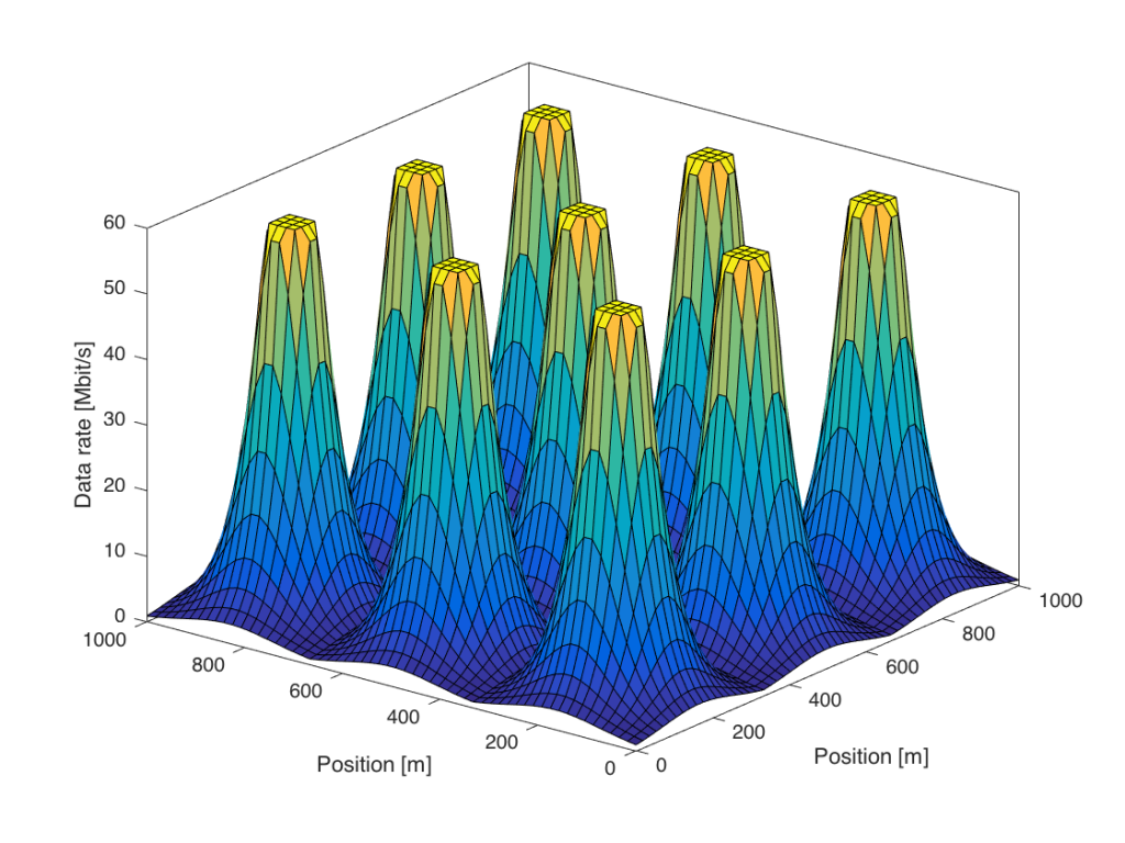
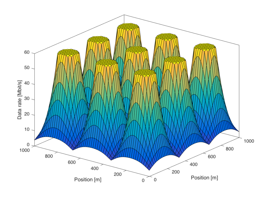
 = bandwidth in Hertz (split equally between uplink and downlink)
 = number of base station antennas
 = number of multiplexed terminals
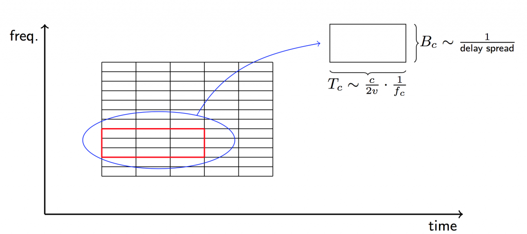
 = coherence bandwidth in Hertz (independent of carrier frequency)
 = coherence time in seconds (inversely proportional to carrier frequency)
 = path loss for the k:th terminal
 = constant, close to
  . The maximal value is
  , which is proportional to
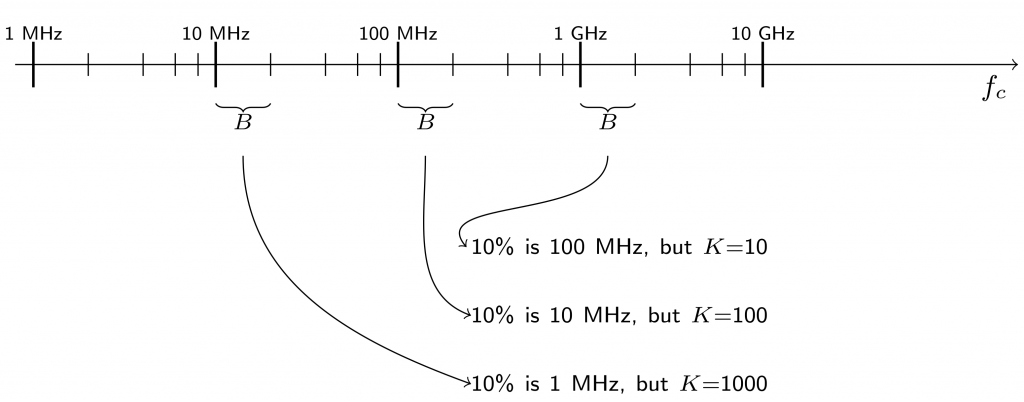

 W is the transmit power,
  is the channel gain, and
  W/Hz is the power spectral density of the noise. The term
  inside the logarithm is referred to as the signal-to-noise ratio (SNR).
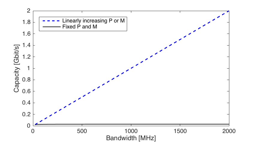
 in the SNR also grows linearly with the bandwidth. This fact is illustrated by Figure 1 below, where we consider a system that achieves an SNR of 0 dB at a reference bandwidth of 20 MHz. As we increase the bandwidth towards 2 GHz, the capacity grows only modestly. Despite the 100 times more bandwidth, the capacity only improves by
  , which is far from the
  that a linear increase would give.
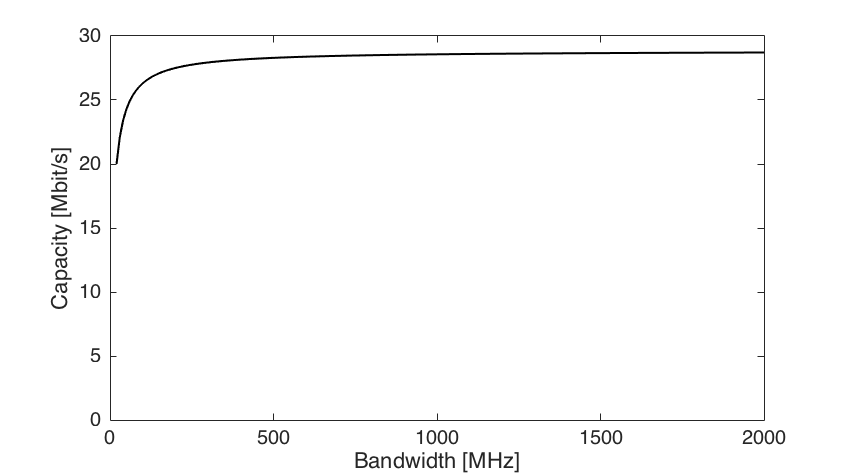

 for
for  .
. , where
  is the gain of a single-antenna channel. Hence, we can increase the number of antennas proportionally to the bandwidth to keep the SNR fixed.