
The channel fading in traditional frequency bands (below 6 GHz) is often well described by the Rayleigh fading model, at least in non-line-of-sight scenarios. This model says that the channel coefficient between any transmit antenna and receive antenna is complex Gaussian distributed, so that its magnitude is Rayleigh distributed.
If there are multiple antennas at the transmitter and/or receiver, then it is common to assume that different pairs of antennas are subject to independent and identically distributed (i.i.d.) fading. This model is called i.i.d. Rayleigh fading and dominates the academic literature to such an extent that one might get the impression that it is the standard case in practice. However, it is rather the other way around: i.i.d. Rayleigh fading only occurs in very special cases in practice, such as having a uniform linear array with half-wavelength-spaced isotropic antennas that is deployed in a rich scattering environment where the multi-paths are uniformly distributed in all directions. If one would remove any of these very specific assumptions then the channel coefficients will become mutually correlated. I covered the basics of spatial correlation in a previous blog post.
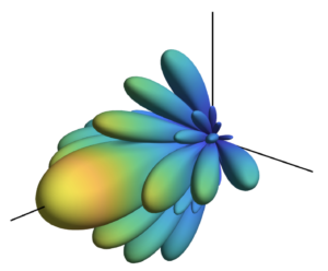
In reality, the channel fading will always be correlated
Some reasons for this are: 1) planar arrays exhibit correlation along the diagonals, since not all adjacent antennas can be half-wavelength-spaced; 2) the antennas have non-isotropic radiation patterns; 3) there will be more multipath components from some directions than from other directions.
With this in mind, I have dedicated a lot of my work to analyzing MIMO communications with correlated Rayleigh fading. In particular, our book “Massive MIMO networks” presents a framework for analyzing multi-user MIMO systems that are subject to correlated fading. When we started the writing, I thought spatial correlation was a phenomenon that was important to cover to match reality but would have a limited impact on the end results. I have later understood that spatial correlation is fundamental to understand how communication systems work. In particular, the modeling of spatial correlation changes the game when it comes to pilot contamination: it is an entirely negative effect under i.i.d. Rayleigh fading models, while a proper analysis based on spatial correlation reveals that one can sometimes benefit from purposely assigning the same pilots to users and then separate them based on their spatial correlation properties.
Future applications for spatial correlation models
The book “Massive MIMO networks” presents a framework for channel estimation and computation of achievable rates with uplink receive combining and downlink precoding for correlated Rayleigh fading channels. Although the title of the book implies that it is about Massive MIMO, the results apply to many beyond-5G research topics. Let me give two concrete examples:
- Cell-free Massive MIMO: In this topic, many geographically distributed access points are jointly serving all the users in the network. This is essentially a single-cell Massive MIMO system where the access points can be viewed as the distributed antennas of a single base station. The channel estimation and computation of achievable rates can be carried out as described “Massive MIMO networks”. The key differences are instead related to which precoding/combining schemes that are considered practically implementable and the reuse of pilots within a cell (which is possible thanks to the strong spatial correlation).
- Extremely Large Aperture Arrays: There are other names for this category, such as holographic MIMO, large intelligent surfaces, and ultra-massive MIMO. The new terminologies are used to indicate the use of co-located arrays that are much larger (in terms of the number of antennas and the physical size) than what is currently considered by the industry when implementing Massive MIMO in 5G. In this case, the spatial correlation matrices must be computed differently than described in “Massive MIMO networks”, for example, to take near-field effects and shadow fading variations into consideration. However, once the spatial correlation matrices have been computed, then the same framework for channel estimation and computation of achievable rates is applicable.
The bottom line is that we can analyze many new exciting beyond-5G technologies by making use of the analytical frameworks developed in the past decade. There is no need to reinvent the wheel but we should reuse as much as possible from previous research and then focus on the novel components. Spatial correlation is something that we know how to deal with and this must not be forgotten.
Hello, Dr. Bjornson.
Your post is very informative and useful as always.
Thank you for sharing.
A question that arise to my mind is that if we have a spatially correlated channel for massive MIMO systems in the real world so this decreases the impact of favourable propagation and maybe this means that we can not assume that the channels between two users are orthogonal anymore. Is this a right idea?
I want to know your opinion.
Thanks.
Favorable propagation behaves differently than in i.i.d. fading. Users that are close to each other (have similar spatial correlation) will exhibit less favorable propagation (more antennas is needed to get the same effect). It is the other way around for users that are far from each other (have very different spatial correlation). I explain this in Section 2 of my book.
However, there is no assumption of channel orthogonality in massive MIMO systems. It is only something that is used in scientific talks to motivate the need for many antennas.
Another question is that do we consider the spatial correlation in massive MIMO systems as an advantage or disadvantage?
It depends on how the users are located. Users that are close to each other (have similar spatial correlation) will get worse performance due to spatial correlation. It is the other way around for users that are far from each other (have very different spatial correlation). There are some examples describing this in Section 2 of my book.
Hello Dr. Björnson ,
May I ask a question? In my opinion, for a cell-free massive MIMO consisting of single-antenna APs and single-antenna UEs, the channel coefficients tend to be uncorrelated because the antennas are distributed and LOS propagation dominates. Is that right?
If yes, when the APs or the UEs have multiple antennas, will the channel model become correlated?
Thank you!
Yes, when considering fading channels, the channel coefficient of different APs are typically modeled uncorrelated.
If an AP has multiple antennas, then those antennas will most likely see correlated realizations of the fading channel.
Sir, it is always interesting to read your blog. Particularly how fading correlation will be beneficial in massive MIMO, which is a key area of my interest. Kindly write more blog posts on this topic.
Regards
-Nirav Patel
Dear Dr. Björnson,
Thanks for your sharing! May I ask a question about the power allocation?
Usually I find in the literatures that the power allocation depends on the large-scale fading. However, for the moving user scenarios in cell-free massive MIMO, the power allocation should be operated dynamically. So my question is how often should the power allocation be performed. If there is some time scale for the power allocation (like the precoding
is performed in each coherence time)?
Kind regards,
Yu
How often the power allocation should be updated depends on how quickly the channel quality varies. The small-scale fading changes in every coherence interval, thus one should ideally update the power allocation in every coherence interval, but that is inconvenient since you need to compute the new powers and inform about them all the time. In a system with a reasonably high level of channel hardening, the small-scale fading variations average out when applying the precoding. The power allocation can then be kept fixed for a longer time period. As long the large-scale fading (i.e., the statistics) remains the same, the power allocation can remain the same.
Dear Dr. Björnson,
Thanks for your replying!
I still have the question: how long the large-scale fading remains the same?
When the users are moving, the positions and the shadowing are always changing, which lead to the large-scale fading changes very quickly. When we consider the power allocation in a cell-free massive MIMO, we should consider the time complexity of the proposed algorithm, the optical processing, ect in practice.
How to ensure a real-time power allocation?
Thanks!
Sincerly, Yu
In theory, the large-scale fading remains the same forever… (This is the underlying assumption when computing achievable rates)
In practice, I have seen measurement results that show that the large-scale fading remains the same for at least 100 x coherence time.
I don’t think it is the changes in large-scale fading that dictates how often the power allocation must be changed in practice but rather the scheduling decisions. When the set of users change, we need to update the power allocation.
Thanks!
Sincerely, Yu
Sir, what is the tapped delay line model in wireless? And please explain the frequency selective model with the tapped delay line model.
thanks.
The wireless channel will contain multiple paths with different time delays. If those delays are large as compared to the symbol time (the time between symbols), then inter-symbol interference appears. This means that you transmit a sequence of symbols, one after the other, but the receiver doesn’t obtain them one after the other. Instead it receives a weighted sum of multiple symbols, where the weights are the “taps”. I recommend you to read Section 2.2.3 in Fundamentals of Wireless Communications, where (2.35) is an example of such a “tapped delay” model. This book is freely available online.
As you increase the bandwidth, the symbol time reduces and you eventually reach a setup with interference between the symbols. This is called frequency selective fading and is also explained in the book mentioned above.
Thank you very much sir for your answer.
Dear Sir, why does the data rate increase with the bandwidth? One of my friend asked me this question today, and I was unable to answer with clarity. Could you please explain this? I googled it but I’m still confused. People relate this with the Shannon capacity theorem. In simple words, as the symbol time decreases, the data rate increases as we can transmit more information within the same interval of time and data rate depends on bandwidth. Please sir explain.
I think you have the answer in your message. I like to relate this to the sampling theorem: The more bandwidth you have, the more sample are needed per second to describe the signal. It is these samples where you put the information, so more samples per second means that more data is delivered per second.
One thing to keep in mind is that the noise power is also proportional to the bandwidth, thus you either need to increase the power proportionally to the bandwidth or live with a gradual SNR reduction as you increase the bandwidth.
Here is a video where I talk about these things: https://youtu.be/kP_FhaclHPg
Thanks, sir, for your answer. Now I understood this crystal clear.
Sir, I have a few more questions.
1. if x(t) and X(f) are Fourier pairs. The bandwidth of X(f) is W Hz and the time spread of x(t) is T secs. Then which of the following could be true.
(a) 0 (b) 0.1 (c)0.001 (d) 20
This question was asked in a Qualcomm written test.
2. y=x+n, where x is BPSK symbol, n is noise which is uniformly distributed between [-2,2]. Then design the optimal detector.
what if noise n is white gaussian?
Sir, I read that in General MAP is better than MLE if prior probabilities are known. Is this true for the case when noise is not Gaussian also?
Thanks in advance sir.
Hi!
1. I think you forgot to state the question. Anyway, I don’t want to provide answers to questions stated in written tests.
2. Generally speaking, MAP is always better or equal to ML. However, MAP reduces to ML when the prior probabilities are equal/uniform. This property focuses on the distribution of the unknown variables (BPSK symbols) and is unrelated to the noise distribution. However, both estimators will change depending on the noise distribution.
Yes sir I forgot to state the question.
Thanks for your reply sir.