

Sometime last week, the paper “Massive MIMO in the UL/DL of Cellular Networks: How Many Antennas Do We Need?” that I have co-authored reached 1000 citations (according to Google Scholar). I feel that this is a good moment to share some reflections on this work and discuss some conclusions we too hastily drew. The paper is an extension of a conference paper that appeared at the 2011 Allerton Conference. At that time, we could by no means anticipate the impact Massive MIMO would have and many people were quite doubtful about the technology (including myself). I still remember very well a heated discussion with an esteemed Bell Lab’s colleague trying to convince me that there were never ever going to be more than two active RF inputs into a base station!
Looking back, I am always wondering where the term “Massive MIMO” actually comes from. When we wrote our paper, the terms “large-scale antenna systems (LSAS)” or simply “large-scale MIMO” were commonly used to refer to base stations with very large antenna arrays, and I do not recall what made us choose our title.
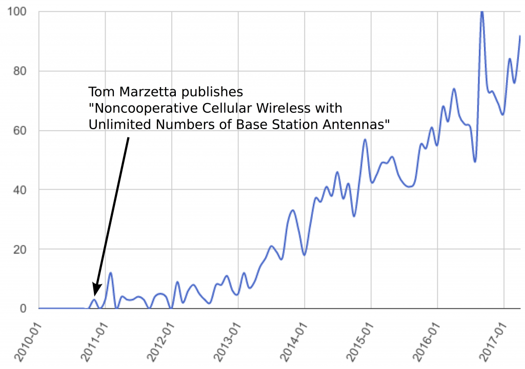
The Google Trends Chart for “Massive MIMO” above clearly shows that interest in this topic started roughly at the time Tom Marzetta’s seminal paper was published, although the term itself does not appear in it at all. If anyone has an idea or reference where the term “Massive MIMO” was first used, please feel free to write this in the comment field.
In case you have not read our paper, let me first explain the key question it tries to answer. Marzetta showed in his paper that the simplest form of linear receive combining and transmit precoding, namely maximum ratio combining (MRC) and transmission (MRT), respectively, achieve an asymptotic spectral efficiency (when the number of antennas goes to infinity) that is only limited by coherent interference caused by user equipments (UEs) using the same pilot sequences for channel training (see the previous blog post on pilot contamination). All non-coherent interference such as noise, channel gain uncertainty due to estimation errors, and interference magically vanishes thanks to the strong law of large numbers and favorable propagation. Intrigued by this beautiful result, we wanted to know what happens for a large but finite number of antennas  . Clearly, MRC/MRT are not optimal in this regime, and we wanted to quantify how much can be gained by using more advanced combining/precoding schemes. In other words, our goal was to figure out how many antennas could be “saved” by computing a matrix inverse, which is the key ingredient of the more sophisticated schemes, such as MMSE combining or regularized zero-forcing (RZF) precoding. Moreover, we wanted to compute how much of the asymptotic spectral efficiency can be achieved with antennas. Please read our paper if you are interested in our findings.
What is interesting to notice is that we (and many other researchers) had always taken the following facts about Massive MIMO for granted and repeated them in numerous papers without further questioning:
- Due to pilot contamination, Massive MIMO has a finite asymptotic capacity
- MRC/MRT are asymptotically optimal
- More sophisticated receive combining and transmit precoding schemes can only improve the performance for finite
We have recently uploaded a new paper on Arxiv which proves that all of these “facts” are incorrect and essentially artifacts from using simplistic channel models and suboptimal precoding/combining schemes. What I find particularly amusing is that we have come to this result by carefully analyzing the asymptotic performance of the multicell MMSE receive combiner that I mentioned but rejected in the 2011 Allerton paper. To understand the difference between the widely used single-cell MMSE (S-MMSE) combining and the (not widely used) multicell MMSE (M-MMSE) combining, let us look at their respective definitions for a base station located in cell  :
:


where  and
and  denote the number of cells and UEs per cell,
  is the estimated channel matrix from the UEs in cell , and
  and
and  are the covariance matrices of the channel and the channel estimation errors of UE
  in cell
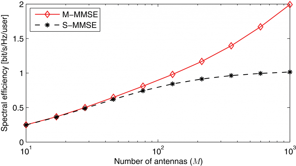
  , respectively. While M-MMSE combining uses estimates of the channels from all UEs in all cells, the simpler S-MMSE combining uses only channel estimates from the UEs in the own cell. Importantly, we show that Massive MIMO with M-MMSE combining has unlimited capacity while Massive MIMO with S-MMSE combining has not! This behavior is shown in the following figure:
In the light of this new result, I wish that we would not have made the following remark in our 2011 Allerton paper:
“Note that a BS could theoretically estimate
all channel matrices(…) to further
improve the performance. Nevertheless, high path loss to
neighboring cells is likely to render these channel estimates unreliable and the potential performance gains are expected to be marginal.”
We could not have been more wrong about it!
In summary, although we did not understand the importance of M-MMSE combining in 2011, I believe that we were asking the right questions. In particular, the consideration of individual channel covariance matrices for each UE has been an important step for the analysis of Massive MIMO systems. A key lesson that I have learned from this story for my own research is that one should always question fundamental assumptions and wisdom.
When Massive MIMO is restricted to per-cell processing, maximum-ratio (MR) and zero-forcing (ZF) perform sufficiently well. (Actually in a multi-cell environment the non-coherent interference tends to dominate such that ZF offers little or no improvement over MR.) Importantly, as we showed in a paper given at the same 2011 Allerton conference, and subsequently in refined form in this textbook, simple and exact formulas exist for the MR and ZF Massive MIMO performance. There is no need to use “deterministic equivalents” or other asymptotic random matrix-theoretic concepts: their mathematics is comparatively difficult, they help propagate the myth that Massive MIMO relies on asymptotics – and, most significantly, the only way of convincing the reader of their accuracy is through simulations (bringing us back to square one).
Regarding multi-cell processing, I too concede that it does appear that the out-of-cell channel responses can be sufficiently well estimated for M-MMSE interference suppression to give real gains. And here, the random-matrix approximations do seem to be the only way forward.
Thank you for your comment, Erik. I fully agree with you that there is no need for any complicated mathematical analysis based on large random matrix theory to study the performance of Massive MIMO under the assumption of uncorrelated fading channels.
However, as soon as one deviates from this assumption, the exact analysis becomes in general intractable and one needs to resort to either Monte Carlo simulations or large system approximations. Simulations are fine if one is only interested in spectral efficiency estimates, but they fail to provide any insight. Large system approximations on the other hand often provide some insight about the most relevant system parameters.
What is very important though is that the asymptotic analyses of the uncorrelated and correlated fading models lead to different conclusions. The former reveals that pilot contamination ultimately limits the performance and MR combining/precoding is asymptotically optimal. The latter indicates that there is no ultimate performance limitation and that M-MMSE combining/precoding is optimal.
Yes. Changing the priors just slightly (and, exploiting them heavily in the Bayesian channel estimation) does seem to change the behavior in the large-number-of-antennas limit dramatically.
Do we know for sure, whether pilot contamination ultimately limits performance in independent Rayleigh fading? Granted, available lower bounds on capacity suggest so, and I conjecture that it does… But are any rigorous upper bounds on capacity available?
This is a good question, in particular the way it is phrased. The question is not if we can get unbounded capacity in such a scenario but rather if pilot contamination is a fundamental limiting factor.
If one allows for time-sharing between cells, i.e., only users in one cell are active at any given time, pilot contamination is non-existent and one gets unbounded capacity for every user as the number of antennas goes to infinity (for any finite number of cells). This holds even for independent Rayleigh fading with MR combining/precoding. However, this is a highly inefficient scheme which one would never use in practice.
If we assume simultaneous transmissions in the cells, pilot contamination necessarily arises and I am not aware of any existing information-theoretic upper bounds. Maybe some area for future research…
Correct: with time-sharing between the cells, capacity scales as ~1/L log(1+M). So for fixed L, Massive MIMO trivially offers “unlimited capacity” when M->infinity even under the canonical independent Rayleigh fading model. This (naive) scheme is exceedingly inefficient for any practical situation and practical M, but it represents a good example of the danger (and here, uselessness) of asymptotic arguments.
This fixed-L assumption is one of the reservations that I have against the conclusions in your recent paper. I do not contest the correctness of the main theorem per se, but it is obtained under the assumption that L is fixed while M->infinity. The more interesting case would be when the limits are interchanged, L->infinity before M->infinity. I conjecture that pilot contamination cannot be overcome in that case, but I do not really know, and I think it is an important open problem.
I don’t think any asymptotic limit is interesting by itself. The important thing is the asymptotic behavior and how it can be used for practical system design. To me, the interesting case is to consider a given setup with a fixed number of cells and users. The challenge is to find a technology that can deliver a given SE of X bit/s/Hz to all users. The naive time-sharing approach would require a huge number of antennas. By mitigating pilot contamination using M-MMSE combining/precoding, as described in our recent work, you need to deploy a much smaller number of antennas. In particular, we show that the M-MMSE approach works in any given setup with any given X:
You tell me how the many users and cells that you have and how many bit/s/Hz/user you need, and I tell you how many antennas do we need
(to paraphrase Hoydis’ seminal paper).
It is interesting to note that M-MMSE interference suppression give gains also in the special case of uncorrelated Rayleigh fading, particularly if there is a pilot reuse factor. The reason is that one can get good estimates of the channels from the strongest interfering users in neighboring cells and use them for interference suppression. These gains might vanish asymptotically, but they are substantial for practical number of antennas. This is what is demonstrated in the simulations of our paper: https://arxiv.org/pdf/1505.03682.pdf
Hi Hoydis,
Is it implied in your paper that the difference between the SINR simulations (when we know the fast-fading channel and pathloss) and SINR approximation (only pathloss known) is small and close to zero?
Do you have any condition how small your difference until it is considered “small” enough?
Does the deterministic equivalent hold for small number of antenna, i.e less than 50 antennas?