The cellular network that my smartphone connects to normally delivers 10-40 Mbit/s. That is sufficient for video-streaming and other applications that I might use. Unfortunately, I sometimes have poor coverage and then I can barely download emails or make a phone call. That is why I think that providing ubiquitous data coverage is the most important goal for 5G cellular networks. It might also be the most challenging 5G goal, because the area coverage has been an open problem since the first generation of cellular technology.
It is the physics that make it difficult to provide good coverage. The transmitted signals spread out and only a tiny fraction of the transmitted power reaches the receive antenna (e.g., one part of a billion parts). In cellular networks, the received signal power reduces roughly as the propagation distance to the power of four. This results in the following data rate coverage behavior:
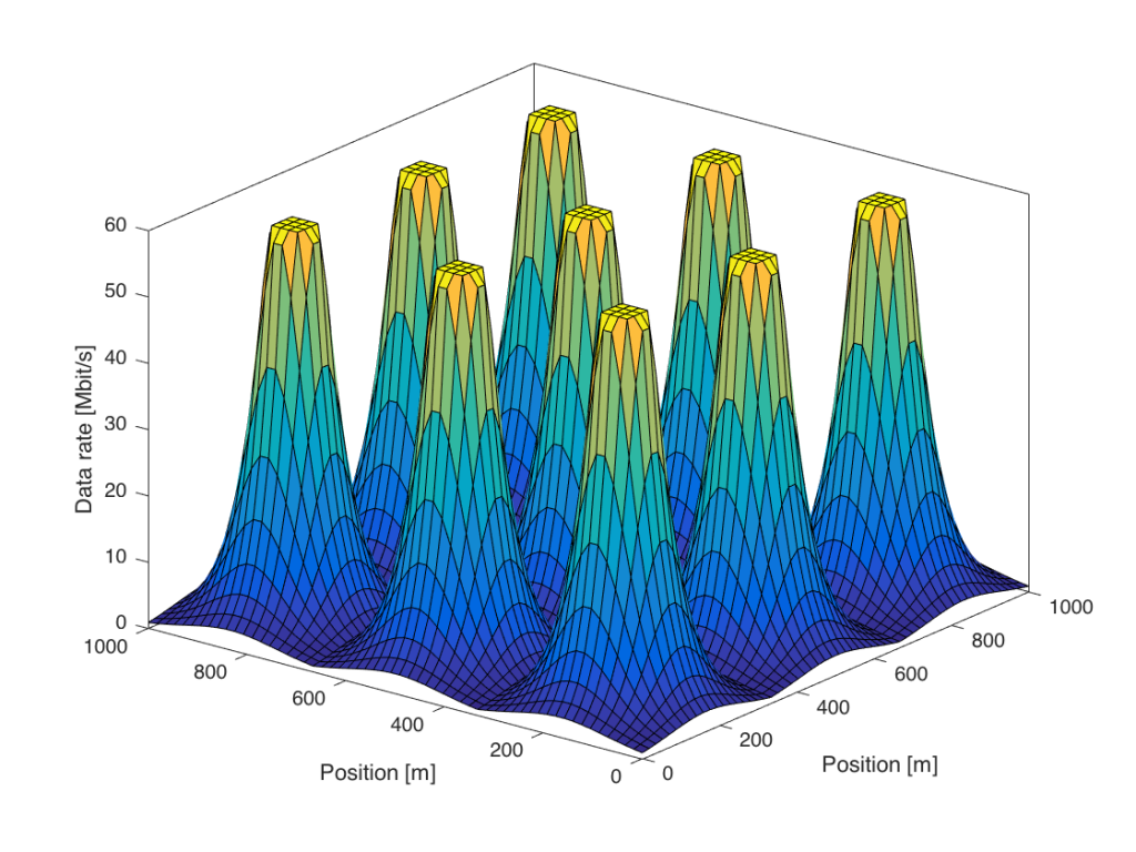
This figure considers an area covered by nine base stations, which are located at the middle of the nine peaks. Users that are close to one of the base stations receive the maximum downlink data rate, which in this case is 60 Mbit/s (e.g., spectral efficiency 6 bit/s/Hz over a 10 MHz channel). As a user moves away from a base station, the data rate drops rapidly. At the cell edge, where the user is equally distant from multiple base stations, the rate is nearly zero in this simulation. This is because the received signal power is low as compared to the receiver noise.
What can be done to improve the coverage?
One possibility is to increase the transmit power. This is mathematically equivalent to densifying the network, so that the area covered by each base station is smaller. The figure below shows what happens if we use 100 times more transmit power:
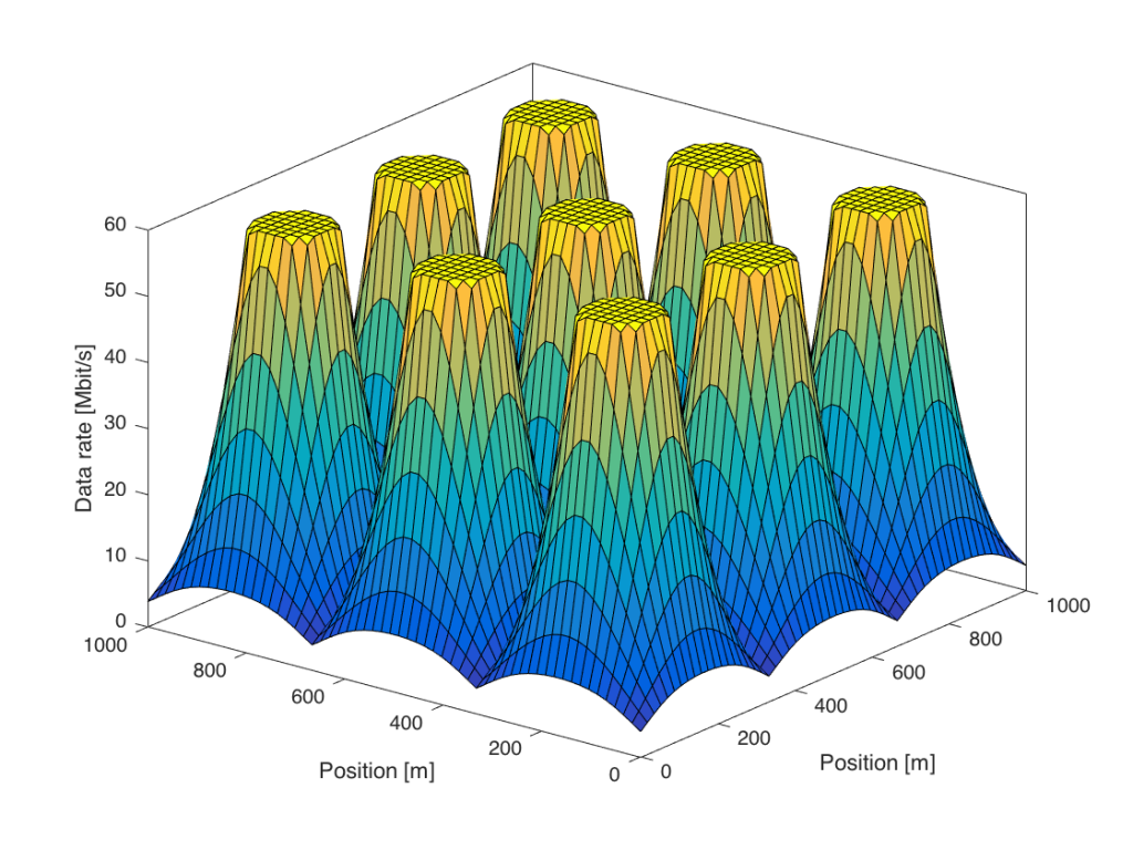
There are some visible differences as compared to Figure 1. First, the region around the base station that gives 60 Mbit/s is larger. Second, the data rates at the cell edge are slightly improved, but there are still large variations within the area. However, it is no longer the noise that limits the cell-edge rates—it is the interference from other base stations.
The inter-cell interference remains even if we would further increase the transmit power. The reason is that the desired signal power as well as the interfering signal power grow in the same manner at the cell edge. Similar things happen if we densify the network by adding more base stations, as nicely explained in a recent paper by Andrews et al.
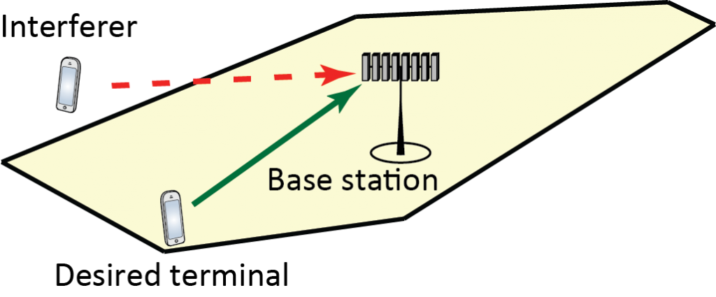
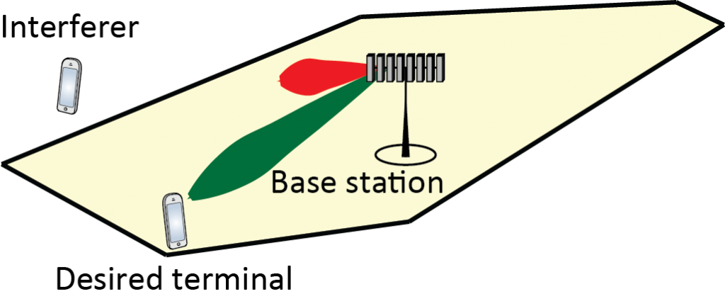
Ideally, we would like to increase only the power of the desired signals, while keeping the interference power fixed. This is what transmit precoding from a multi-antenna array can achieve; the transmitted signals from the multiple antennas at the base station add constructively only at the spatial location of the desired user. More precisely, the signal power is proportional to M (the number of antennas), while the interference power caused to other users is independent of M. The following figure shows the data rates when we go from 1 to 100 antennas:
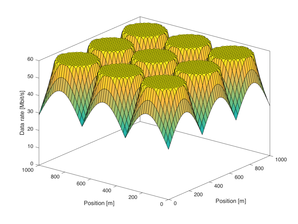
Figure 3 shows that the data rates are increased for all users, but particularly for those at the cell edge. In this simulation, everyone is now guaranteed a minimum data rate of 30 Mbit/s, while 60 Mbit/s is delivered in a large fraction of the coverage area.
In practice, the propagation losses are not only distant-dependent, but also affected by other large-scale effects, such as shadowing. The properties described above remain nevertheless. Coherent precoding from a base station with many antennas can greatly improve the data rates for the cell edge users, since only the desired signal power (and not the interference power) is increased. Higher transmit power or smaller cells will only lead to an interference-limited regime where the cell-edge performance remains to be poor. A practical challenge with coherent precoding is that the base station needs to learn the user channels, but reciprocity-based Massive MIMO provides a scalable solution to that. That is why Massive MIMO is the key technology for delivering ubiquitous connectivity in 5G.
 Hz. By assuming an additive white Gaussian noise channel, the capacity becomes
 W is the transmit power,
  is the channel gain, and
  W/Hz is the power spectral density of the noise. The term
  inside the logarithm is referred to as the signal-to-noise ratio (SNR).
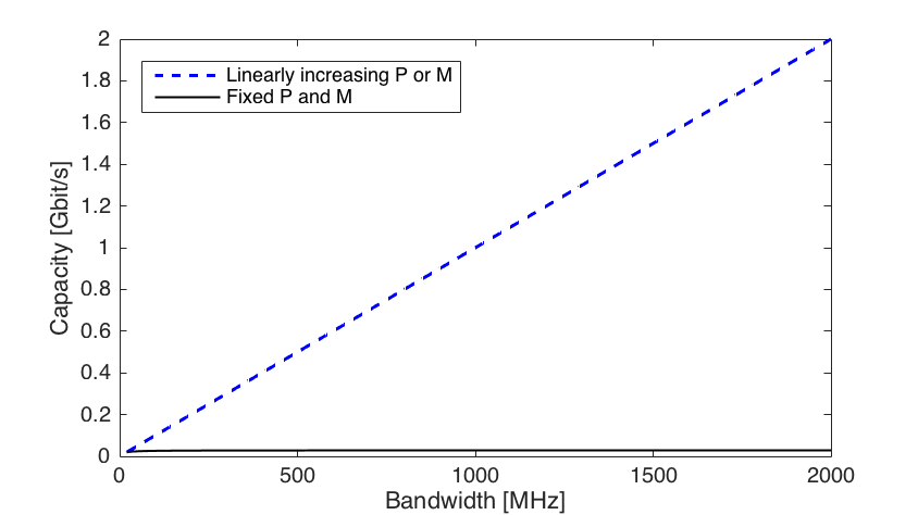
 in the SNR also grows linearly with the bandwidth. This fact is illustrated by Figure 1 below, where we consider a system that achieves an SNR of 0 dB at a reference bandwidth of 20 MHz. As we increase the bandwidth towards 2 GHz, the capacity grows only modestly. Despite the 100 times more bandwidth, the capacity only improves by
  , which is far from the
  that a linear increase would give.
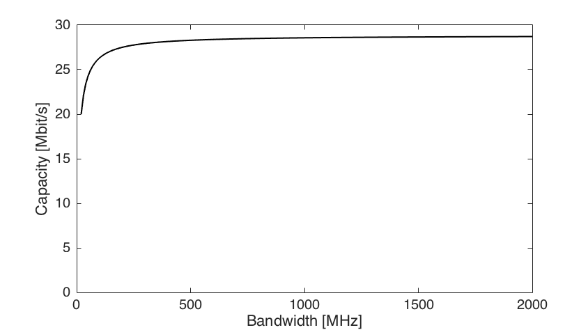

 for
for  .
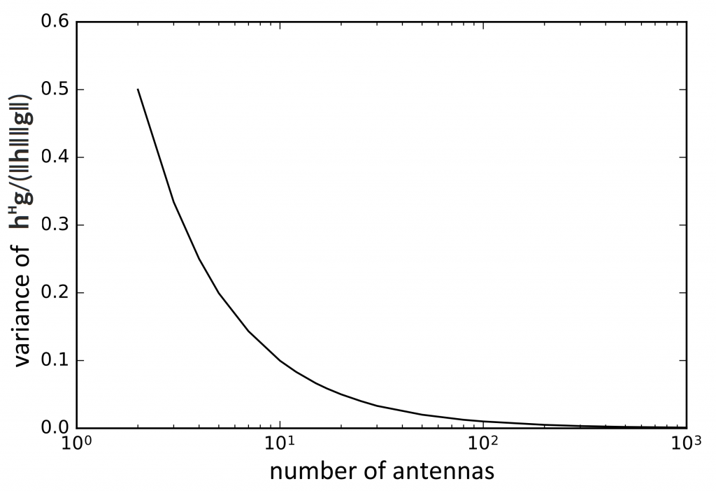
. , where
  is the number of antennas and
  is the gain of a single-antenna channel. Hence, we can increase the number of antennas proportionally to the bandwidth to keep the SNR fixed.