
The received signal power is proportional to the number of antennas  in Massive MIMO systems. This property is known as the array gain and it can basically be utilized in two different ways.
One option is to let the signal power become times larger than in a single-antenna reference scenario. The increase in SNR will then lead to higher data rates for the users. The gain can be anything from  bit/s/Hz to almost negligible, depending on how interference-limited the system is. Another option is to utilize the array gain to reduce the transmit power, to maintain the same SNR as in the reference scenario. The corresponding power saving can be very helpful to improve the energy efficiency of the system.
In the uplink, with single-antenna user terminals, we can choose between these options. However, in the downlink, we might not have a choice. There are strict regulations on the permitted level of out-of-band radiation in practical systems. Since Massive MIMO uses downlink precoding, the transmitted signals from the base station have a stronger directivity than in the single-antenna reference scenario. The signal components that leak into the bands adjacent to the intended frequency band will then also be more directive.
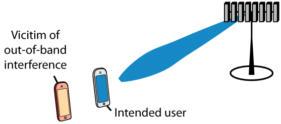
For example, consider a line-of-sight scenario where the precoding creates an angular beam towards the intended user (as illustrated in the figure below). The out-of-band radiation will then get a similar angular directivity and lead to larger interference to systems operating in adjacent bands, if their receivers are close to the user (as the victim in the figure below). To counteract this effect, our only choice might be to reduce the downlink transmit power to keep the worst-case out-of-band radiation constant.
Another alternative is that the regulations are made more flexible with respect to precoded transmissions. The probability that a receiver in an adjacent band is hit by an interfering out-of-band beam, such that the interference becomes times larger than in the reference scenario, reduces with an increasing number of antennas since the beams are narrower. Hence, if one can allow for beamformed out-of-band interference if it occurs with sufficiently low probability, the array gain in Massive MIMO can still be utilized to increase the SNRs. A third option will then be to (partially) reduce the transmit power to also allow for relaxed linearity requirements of the hardware.
These considerations are nicely discussed in an overview article that appeared on ArXiv earlier this year. There are also two papers that analyze the impact of out-of-bound radiation in Massive MIMO: Paper 1 and Paper 2.


 . Massive MIMO is so tightly connected with asymptotic analysis that reviewers question whether a paper is actually about Massive MIMO if it does not contain an asymptotic part – this has happened to me repeatedly.
 and still approach a non-zero asymptotic rate limit. This type of scaling law has been derived for many different scenarios in different papers. The practical implication is that you can reduce the transmit power as you add more antennas, but the asymptotic scaling law does not prescribe how much you should reduce the power when going from, say, 40 to 400 antennas. It all depends on which rates you want to deliver to your users.
 antennas, the transmit power per antenna is just 1 mW, which is unnecessarily low given the fact that the circuits in the corresponding transceiver chain will consume much more power. By using higher transmit power than 1 mW per antenna, we can deliver higher rates to the users, while barely effecting the total power of the base station.
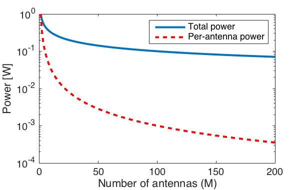
 and approach a non-zero asymptotic rate limit. The practical implication is that Massive MIMO systems can use simpler hardware components (that cause more distortion) than conventional systems, since there is a lower sensitivity to distortion. This is the foundation on which the recent works on low-bit ADC resolutions builds (
 , where
  is the variance.
 has an
  -distribution (this is a scaled
  distribution) and the channel direction
  is uniformly distributed over the unit sphere in
  . The channel gain and the channel direction are also independent random variables, which is why this is a spatially uncorrelated channel model.
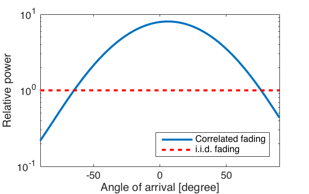
 , where the covariance matrix
  is also the correlation matrix. It is only when
  . The fraction of strong eigenvalues is related to the fraction of the angular interval from which strong signals are received.
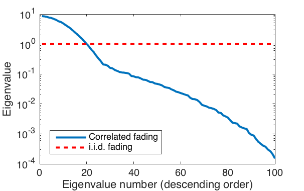
 , where the mean value
  represents the deterministic line-of-sight channel and the covariance matrix
  can still be used to determine the spatial correlation of the received signal power. However, from a system performance perspective, the fraction
  between the power of the line-of-sight path and the scattered paths can have a large impact on the performance as well. A nearly deterministic channel with a large
  -factor provide more reliable communication, in particular since under correlated fading it is only the large eigenvalues of
 The 5G Myth is the provocative title of a recent book by