What is the Difference Between Beamforming and Precoding?

I’ve got an email with this question last week. There is not one but many possible answers to this question, so I figured that I write a blog post about it.

One answer is that beamforming and precoding are two words for exactly the same thing, namely to use an antenna array to transmit one or multiple spatially directive signals.

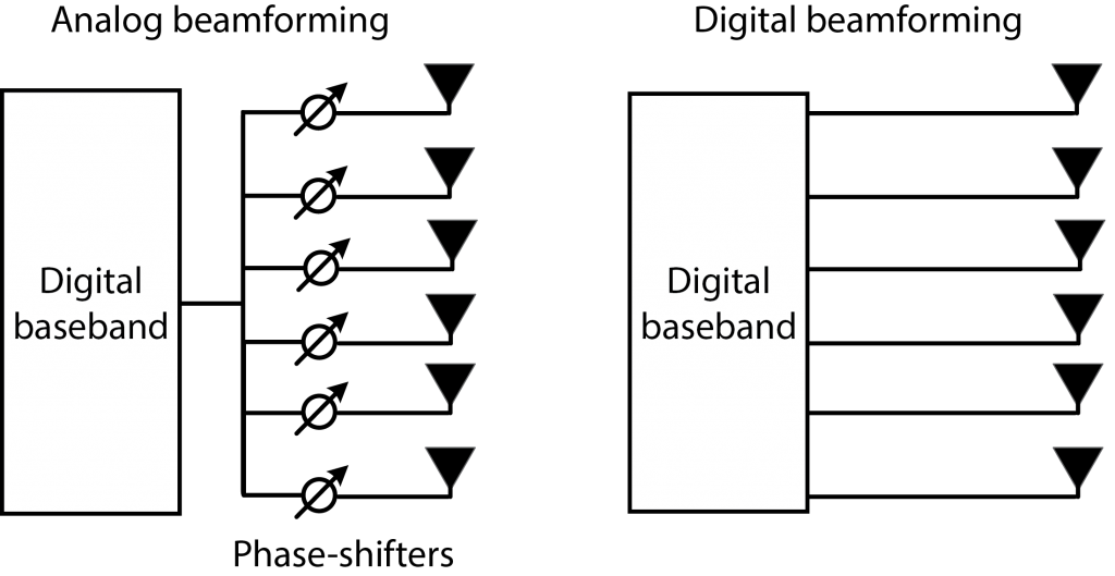
Another answer is that beamforming can be divided into two categories: analog and digital beamforming. In the former category, the same signal is fed to each antenna and then analog phase-shifters are used to steer the signal emitted by the array. This is what a phased array would do. In the latter category, different signals are designed for each antenna in the digital domain. This allows for greater flexibility since one can assign different powers and phases to different antennas and also to different parts of the frequency bands (e.g., subcarriers). This makes digital beamforming particularly desirable for spatial multiplexing, where we want to transmit a superposition of signals, each with a separate directivity. It is also beneficial when having a wide bandwidth because with fixed phases the signal will get a different directivity in different parts of the band. The second answer to the question is that precoding is equivalent to digital beamforming. Some people only mean analog beamforming when they say beamforming, while others use the terminology for both categories.

Analog beamforming uses phase-shifters to send the same signal from multiple antennas but with different phases. Digital beamforming designs different signals for each antennas in the digital baseband. Precoding is sometimes said to be equivalent to digital beamforming.

A third answer is that beamforming refers to a single-user transmission with one data stream, such that the transmitted signal consists of one main-lobe and some undesired side-lobes. In contrast, precoding refers to the superposition of multiple beams for spatial multiplexing of several data streams.

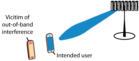
A fourth answer is that beamforming refers to the formation of a beam in a particular angular direction, while precoding refers to any type of transmission from an antenna array. This definition essentially limits the use of beamforming to line-of-sight (LoS) communications, because when transmitting to a non-line-of-sight (NLoS) user, the transmitted signal might not have a clear angular directivity. The emitted signal is instead matched to the multipath propagation so that the multipath components that reach the user add constructively.

A fifth answer is that precoding consists of two parts: choosing the directivity (beamforming) and choosing the transmit power (power allocation).

I used to use the word beamforming in its widest meaning (i.e., the first answer), as can be seen in my first book on the topic. However, I have since noticed that some people have a more narrow or specific interpretation of beamforming. Therefore, I nowadays prefer only talking about precoding. In Massive MIMO, I think that precoding is the right word to use since what I advocate is a fully digital implementation, where the phases and powers can be jointly designed to achieve high capacity through spatial multiplexing of many users, in both NLoS and LOS scenarios.

Six Differences Between Massive MIMO for Sub-6 GHz and mmWave

The “Massive MIMO” name is currently being used for both sub-6 GHz and mmWave applications. This can be very confusing because the multi-antenna technology has rather different characteristics in these two applications.

The sub-6 GHz spectrum is particularly useful to provide network coverage, since the pathloss and channel coherence time are relatively favorable at such frequencies (recall that the coherence time is inversely proportional to the carrier frequency). Massive MIMO at sub-6 GHz spectrum can increase the efficiency of highly loaded cells, by upgrading the technology at existing base stations. In contrast, the huge available bandwidths in mmWave bands can be utilized for high-capacity services, but only over short distances due to the severe pathloss and high noise power (which is proportional to the bandwidth). Massive MIMO in mmWave bands can thus be used to improve the link budget.

Six key differences between sub-6 GHz and mmWave operation are provided below:

Sub-6 GHz mmWave
Deployment scenario Macro cells with support for high user mobility Small cells with low user mobility
Number of simultaneous users per cell Up to tens of users, due to the large coverage area One or a few users, due to the small coverage area
Main benefit from having many antennas Spatial multiplexing of tens of users, since the array gain and ability to separate users spatially lead to great spectral efficiency Beamforming to a single user, which greatly improves the link budget and thereby extends coverage
Channel characteristics Rich multipath propagation Only a few propagation paths
Spectral efficiency and bandwidth High spectral efficiency due to the spatial multiplexing, but small bandwidth Low spectral efficiency due to few users, large pathloss, and large noise power, but large bandwidth
Transceiver hardware Fully digital transceiver implementations are feasible and have been prototyped Hybrid analog-digital transceiver implementations are needed, at least in the first products

Since Massive MIMO was initially proposed by Tom Marzetta for sub-6 GHz applications, I personally recommend to use the “Massive MIMO” name  only for that use case. One can instead say “mmWave Massive MIMO” or just “mmWave” when referring to multi-antenna technologies for mmWave bands.

5.5 Hours of Massive MIMO Tutorials

Video recordings from the 2017 Joint IEEE SPS and EURASIP Summer School on Signal Processing for 5G Wireless Access are available for IEEE members, as we wrote about in a previous post. Now two of the Massive MIMO tutorial talks are openly available on Youtube.

Prof. Erik. G. Larsson gave a 2.5 hour tutorial on the fundamentals of Massive MIMO, which is highly recommended for anyone learning this topic. You can then follow up by reading his book with the same topic.

When you have viewed Erik’s introduction, you can learn more about the state-of-the-art signal processing schemes for Massive MIMO from another talk at the summer school. Dr. Emil Björnson gave a 3 hour tutorial on this topic:

Out-of-band Radiation can Impact the Massive MIMO Operation

The received signal power is proportional to the number of antennas M in Massive MIMO systems. This property is known as the array gain and it can basically be utilized in two different ways.

One option is to let the signal power become M times larger than in a single-antenna reference scenario. The increase in SNR will then lead to higher data rates for the users. The gain can be anything from \log_2(M) bit/s/Hz to almost negligible, depending on how interference-limited the system is. Another option is to utilize the array gain to reduce the transmit power, to maintain the same SNR as in the reference scenario. The corresponding power saving can be very helpful to improve the energy efficiency of the system.

In the uplink, with single-antenna user terminals, we can choose between these options. However, in the downlink, we might not have a choice. There are strict regulations on the permitted level of out-of-band radiation in practical systems. Since Massive MIMO uses downlink precoding, the transmitted signals from the base station have a stronger directivity than in the single-antenna reference scenario. The signal components that leak into the bands adjacent to the intended frequency band will then also be more directive.

For example, consider a line-of-sight scenario where the precoding creates an angular beam towards the intended user (as illustrated in the figure below). The out-of-band radiation will then get a similar angular directivity and lead to larger interference to systems operating in adjacent bands, if their receivers are close to the user (as the victim in the figure below). To counteract this effect, our only choice might be to reduce the downlink transmit power to keep the worst-case out-of-band radiation constant.

Another alternative is that the regulations are made more flexible with respect to precoded transmissions. The probability that a receiver in an adjacent band is hit by an interfering out-of-band beam, such that the interference becomes M times larger than in the reference scenario, reduces with an increasing number of antennas since the beams are narrower. Hence, if one can allow for beamformed out-of-band interference if it occurs with sufficiently low probability, the array gain in Massive MIMO can still be utilized to increase the SNRs. A third option will then be to (partially) reduce the transmit power to also allow for relaxed linearity requirements of the hardware.

These considerations are nicely discussed in an overview article that appeared on ArXiv earlier this year. There are also two papers that analyze the impact of out-of-bound radiation in Massive MIMO: Paper 1 and Paper 2.

Asymptomania

I am borrowing the title from a column written by my advisor two decades ago, in the array signal processing gold rush era.

Asymptotic analysis is a popular tool within statistical signal processing (infinite SNR or number of samples), information theory (infinitely long blocks) and more recently, [massive] MIMO wireless communications (infinitely many antennas).

Some caution is strongly advisable with respect to the latter. In fact, there are compelling reasons to avoid asymptotics in the number of antennas altogether:

  • First, elegant, rigorous and intuitively comprehensible capacity bound formulas are available in closed form.
    The proofs of these expressions use basic random matrix theory, but no asymptotics at all.
  • Second, the notion of “asymptotic limit” or “asymptotic behavior” helps propagate the myth that Massive MIMO somehow relies on asymptotics or “infinite” numbers (or even exorbitantly large numbers) of antennas.
  • Third, many approximate performance results for Massive MIMO (particularly “deterministic equivalents”) based on asymptotic analysis are complicated, require numerical evaluation, and offer little intuitive insight. (And, the verification of their accuracy is a formidable task.)

Finally, and perhaps most importantly, careless use of asymptotic arguments may yield erroneous conclusions. For example in the effective SINRs in multi-cell Massive MIMO, the coherent interference scales with M (number of antennas) – which yields the commonly held misconception that coherent interference is the main impairment caused by pilot contamination. But in fact, in many relevant circumstances it is not (see case studies here): the main impairment for “reasonable” values of M is the reduction in coherent beamforming gain due to reduced estimation quality, which in turn is independent of M.

In addition, the number of antennas beyond which the far-field assumption is violated is actually smaller than what one might first think (problem 3.14).

IEEE ComSoc Focuses on Massive MIMO

IEEE ComSoc provides new online material every month and in August the focus is on Massive MIMO.

First, four carefully selected articles are offered free of charge, see the screenshot below and click here for details.

More precisely, IEEE offers free access to the published versions of these articles, while the accepted versions were already openly available: Paper 1, Paper 2, Paper 3, and Paper 4.

Second, a live webinar entitled “5G Massive MIMO: Achieving Spectrum Efficiency” is organized by IEEE ComSoc on August 24. The speaker is Professor Liesbet Van der Perre from KU Leuven. She was the scientific leader of the MAMMOET project, which is famous for demonstrating that Massive MIMO works in practice. You can expect a unique mix of theoretical concepts and practical implementation insights from this webinar.

News – commentary – mythbusting