What is the Purpose of Asymptotic Analysis?

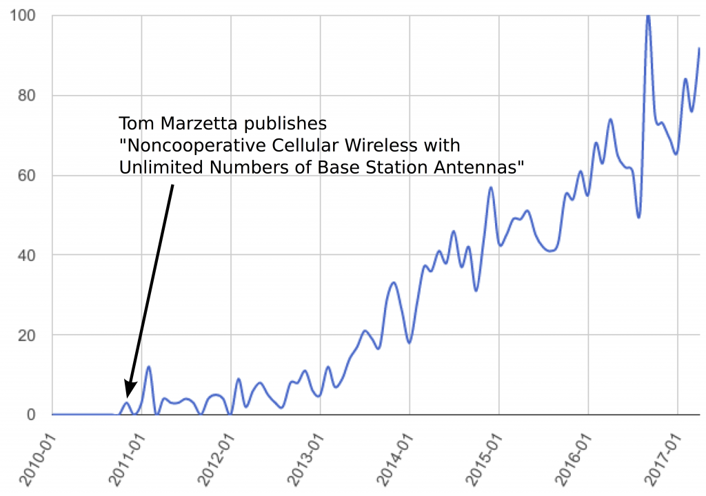
Since its inception, Massive MIMO has been strongly connected with asymptotic analysis. Marzetta’s seminal paper featured an unlimited number of base station antennas. Many of the succeeding papers considered a finite number of antennas, M, and then analyzed the performance in the limit where M\to\infty. Massive MIMO is so tightly connected with asymptotic analysis that reviewers question whether a paper is actually about Massive MIMO if it does not contain an asymptotic part – this has happened to me repeatedly.

Have you reflected over what the purpose of asymptotic analysis is? The goal is not that we should design and deploy wireless networks with a nearly infinite number of antennas. Firstly, it is physically impossible to do that in a finite-sized world, irrespective of whether you let the array aperture grow or pack the antennas more densely. Secondly, the conventional channel models break down, since you will eventually receive more power than you transmitted. Thirdly, the technology will neither be cost nor energy efficient, since the cost/energy grows linearly with M, while the delivered system performance either approaches a finite limit or grows logarithmically with M.

It is important not to overemphasize the implications of asymptotic results. Consider the popular power-scaling law which says that one can use the array gain of Massive MIMO to reduce the transmit power as 1/\sqrt{M} and still approach a non-zero asymptotic rate limit. This type of scaling law has been derived for many different scenarios in different papers. The practical implication is that you can reduce the transmit power as you add more antennas, but the asymptotic scaling law does not prescribe how much you should reduce the power when going from, say, 40 to 400 antennas. It all depends on which rates you want to deliver to your users.

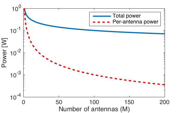
The figure below shows the transmit power in a scenario where we start with 1 W for a single-antenna transmitter and then follow the asymptotic power-scaling law as the number of antennas increases. With M=100 antennas, the transmit power per antenna is just 1 mW, which is unnecessarily low given the fact that the circuits in the corresponding transceiver chain will consume much more power. By using higher transmit power than 1 mW per antenna, we can deliver higher rates to the users, while barely effecting the total power of the base station.

Reducing the transmit power per antenna to 1 mW, or smaller, makes little practical sense, since the transceiver chain will consume much more power irrespective of the transmit power.

Similarly, there is a hardware-scaling law which says that one can increase the error vector magnitude (EVM) proportionally to M^{1/4} and approach a non-zero asymptotic rate limit. The practical implication is that Massive MIMO systems can use simpler hardware components (that cause more distortion) than conventional systems, since there is a lower sensitivity to distortion. This is the foundation on which the recent works on low-bit ADC resolutions builds (see this paper and references therein).

Even the importance of the coherent interference, caused by pilot contamination, is easily overemphasized if one only considers the asymptotic behavior.  For example, the finite rate limit that appears when communicating over i.i.d. Rayleigh fading channels with maximum ratio or zero-forcing processing is only approached in practice if one has around one million antennas.

In my opinion, the purpose of asymptotic analysis is not to understand the asymptotic behaviors themselves, but what the asymptotics can tell us about the performance at practical number of antennas. Here are some usages that I think are particularly sound:

  • Determine what is the asymptotically optimal transmission scheme and then evaluate how it performs in a practical system.
  • Derive large-scale approximations of the rates that are reasonable tight also at practical number of antennas. One can use these approximations to determine which factors that have a dominant impact on the rate or to get a tractable way to optimize system performance (e.g., by transmit power allocation).
  • Determine how far from the asymptotically achievable performance a practical system is.
  • Determine if we can deliver any given user rates by simply deploying enough antennas, or if the system is fundamentally interference limited.
  • Simplify the signal processing by utilizing properties such as channel hardening and favorable propagation. These phenomena can be observed already at 100 antennas, although you will never get a fully deterministic channel or zero inter-user interference in practice.

Some form of Massive MIMO will appear in 5G, but to get a well-designed system we need to focus more on demonstrating and optimizing the performance in practical scenarios (e.g., the key 5G use cases) and less on pure asymptotic analysis.

What is Spatial Channel Correlation?

The channel between a single-antenna user and an M-antenna base station can be represented by an M-dimensional channel vector. The canonical channel model in the Massive MIMO literature is independent and identically distributed (i.i.d.) Rayleigh fading, in which the vector is a circularly symmetric complex Gaussian random variable with a scaled identity matrix as correlation/covariance matrix: \mathbf{h} \sim CN(\mathbf{0},\beta \mathbf{I}_M), where \beta is the variance.

With i.i.d. Rayleigh fading, the channel gain \|\mathbf{h}\|^2 has an Erlang(M,1/\beta)-distribution (this is a scaled \chi^2 distribution) and the channel direction \mathbf{h} / \|\mathbf{h}\| is uniformly distributed over the unit sphere in \mathbb{C}^M. The channel gain and the channel direction are also independent random variables, which is why this is a spatially uncorrelated channel model.

One of the key benefits of i.i.d. Rayleigh fading is that one can compute closed-form rate expressions, at least when using maximum ratio or zero-forcing processing; see Fundamentals of Massive MIMO for details. These expressions have an intuitive interpretation, but should be treated with care because practical channels are not spatially uncorrelated. Firstly, due to the propagation environment, the channel vector is more probable to point in some directions than in others. Secondly, the antennas have spatially dependent antenna patterns. Both factors contribute to the fact that spatial channel correlation always appears in practice.

One of the basic properties of spatial channel correlation is that the base station array receives different average signal power from different spatial directions. This is illustrated in Figure 1 below for a uniform linear array with 100 antennas, where the angle of arrival is measured from the boresight of the array.

Figure 1: The average signal power received at a Massive MIMO base station from different angular directions, as seen from the array. Spatially correlated fading implies that this average power is angle-dependent, while i.i.d. fading gives the same power in all directions.


As seen from Figure 1, with i.i.d. Rayleigh fading the average received power is equally large from all directions, while with spatially correlated fading it varies depending on in which direction the base station applies its receive beamforming. Note that this is a numerical example that was generated by letting the signal come from four scattering clusters located in different angular directions. Channel measurements from Lund University (see Figure 4 in this paper) show how the spatial correlation behaves in practical scenarios.

Correlated Rayleigh fading is a tractable way to model a spatially  correlation channel vector: \mathbf{h} \sim CN(\mathbf{0}, \mathbf{B})
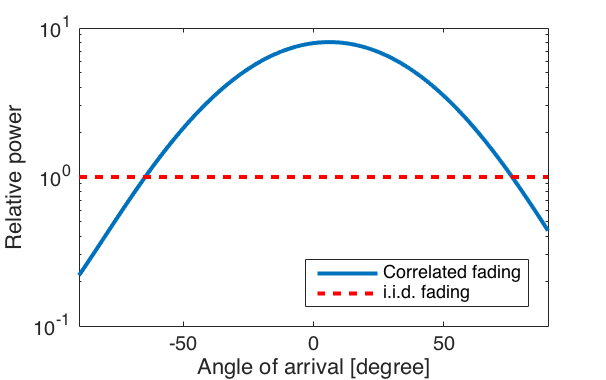
, where the covariance matrix \mathbf{B} is also the correlation matrix. It is only when \mathbf{B} is a scaled identity matrix that we have spatially uncorrelated fading. The eigenvalue distribution determines how strongly spatially correlated the channel is. If all eigenvalues are identical, then \mathbf{B} is a scaled identity matrix and there is no spatial correlation. If there are a few strong eigenvalues that contain most of the power, then there is very strong spatial correlation and the channel vector is very likely to be (approximately) spanned by the corresponding eigenvectors. This is illustrated in Figure 2 below, for the same scenario as in the previous figure. In the considered correlated fading case, there are 20 eigenvalues that are larger than in the i.i.d. fading case. These eigenvalues contain 94% of the power, while the next 20 eigenvalues contain 5% and the smallest 60 eigenvalues only contain 1%. Hence, most of the power is concentrated to a subspace of dimension \leq40. The fraction of strong eigenvalues is related to the fraction of the angular interval from which strong signals are received. This relation can be made explicit in special cases.

Figure 2: Spatial channel correlation results in eigenvalue variations, while all eigenvalues are the same under i.i.d fading. The larger the variations, the stronger the correlation is.


One example of spatially correlated fading is when the correlation matrix has equal diagonal elements and non-zero off-diagonal elements, which describe the correlation between the channel coefficients of different antennas. This is a reasonable model when deploying a compact base station array in tower. Another example is a diagonal correlation matrix with different diagonal elements. This is a reasonable model when deploying distributed antennas, as in the case of cell-free Massive MIMO.

Finally, a more general channel model is correlated Rician fading: \mathbf{h} \sim CN(\mathbf{b}, \mathbf{B})
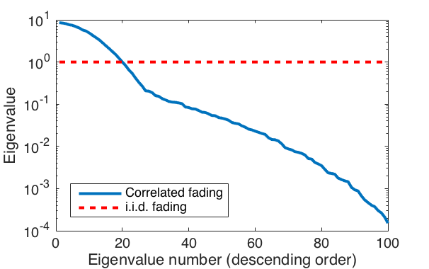
, where the mean value \mathbf{b} represents the deterministic line-of-sight channel and the covariance matrix \mathbf{B} determines the properties of the fading. The correlation matrix \mathbf{B}+\mathbf{b}\mathbf{b}^H can still be used to determine the spatial correlation of the received signal power. However, from a system performance perspective, the fraction k=\| \mathbf{b} \|^2/\mathrm{tr}(\mathbf{B}) between the power of the line-of-sight path and the scattered paths can have a large impact on the performance as well. A nearly deterministic channel with a large  k-factor provide more reliable communication, in particular since under correlated fading it is only the large eigenvalues of \mathbf{B} that contributes to the channel hardening (which otherwise provides reliability in Massive MIMO).

Reflections on “Massive MIMO: How Many Antennas Do We Need?”

Sometime last week, the paper “Massive MIMO in the UL/DL of Cellular Networks: How Many Antennas Do We Need?”  that I have co-authored  reached 1000 citations (according to Google Scholar). I feel that this is a good moment to share some reflections on this work and discuss some conclusions we too hastily drew. The paper is an extension of a conference paper that appeared at the 2011 Allerton Conference. At that time, we could by no means anticipate the impact Massive MIMO would have and many people were quite doubtful about the technology (including myself). I still remember very well a heated discussion with an esteemed Bell Lab’s colleague trying to convince me that there were never ever going to be more than two active RF inputs into a base station!

Looking back, I am always wondering where the term “Massive MIMO” actually comes from. When we wrote our paper, the terms “large-scale antenna systems (LSAS)” or simply “large-scale MIMO” were commonly used to refer to base stations with very large antenna arrays, and I do not recall what made us choose our title.

The Google Trends Chart for “Massive MIMO” above clearly shows that interest in this topic started roughly at the time Tom Marzetta’s seminal paper was published, although the term itself does not appear in it at all. If anyone has an idea or reference where the term “Massive MIMO” was first used, please feel free to write this in the comment field.

In case you have not read our paper, let me first explain the key question it tries to answer. Marzetta showed in his paper that the simplest form of linear receive combining and transmit precoding, namely maximum ratio combining (MRC) and transmission (MRT), respectively, achieve an asymptotic spectral efficiency (when the number of antennas goes to infinity) that is only limited by coherent interference caused by user equipments (UEs) using the same pilot sequences for channel training (see the previous blog post on pilot contamination). All non-coherent interference such as noise, channel gain uncertainty due to estimation errors, and interference magically vanishes thanks to the strong law of large numbers and favorable propagation. Intrigued by this beautiful result, we wanted to know what happens for a large but finite number of antennas M. Clearly, MRC/MRT are not optimal in this regime, and we wanted to quantify how much can be gained by using more advanced combining/precoding schemes. In other words, our goal was to figure out how many antennas could be “saved” by computing a matrix inverse, which is the key ingredient of the more sophisticated schemes, such as MMSE combining or regularized zero-forcing (RZF) precoding. Moreover, we wanted to compute how much of the asymptotic spectral efficiency can be achieved with M antennas. Please read our paper if you are interested in our findings.

What is interesting to notice is that we (and many other researchers) had always taken the following facts about Massive MIMO for granted and repeated them in numerous papers without further questioning:

  • Due to pilot contamination, Massive MIMO has a finite asymptotic capacity
  • MRC/MRT are asymptotically optimal
  • More sophisticated receive combining and transmit precoding schemes can only improve the performance for finite M

We have recently uploaded a new paper on Arxiv which proves that all of these “facts” are incorrect and essentially artifacts from using simplistic channel models and suboptimal precoding/combining schemes. What I find particularly amusing is that we have come to this result by carefully analyzing the asymptotic performance of the multicell MMSE receive combiner that I mentioned but rejected in the 2011 Allerton paper. To understand the difference between the widely used single-cell MMSE (S-MMSE) combining and the (not widely used) multicell MMSE (M-MMSE) combining, let us look at their respective definitions for a base station located in cell j:

\mathbf{V}^{\textrm{M-MMSE}}_j = \left( \sum_{l=1}^{L} \hat{\mathbf{H}}_l \hat{\mathbf{H}}_l^H + \sum_{l=1}^L \sum_{i=1}^K \mathbf{C}_{li} + \sigma^2 \mathbf{I}_M \right)^{-1} \hat{\mathbf{H}}_{j}

\mathbf{V}^{\textrm{S-MMSE}}_j = \left( \hat{\mathbf{H}}_j \hat{\mathbf{H}}_j^H + \sum_{i=1}^K \mathbf{C}_{ji} + \sum_{l=1, l\neq j}^L \sum_{i=1}^K \mathbf{R}_{li} + \sigma^2 \mathbf{I}_M \right)^{-1} \hat{\mathbf{H}}_{j}

where L and K denote the number of cells and UEs per cell, \hat{\mathbf{H}}_j\in \mathbb{C}^{M\times K} is the estimated channel matrix from the UEs in cell j, and \mathbf{R}_{li} and \mathbf{C}_{li} are the covariance matrices of the channel and the channel estimation errors of UE i in cell l, respectively. While M-MMSE combining uses estimates of the channels from all UEs in all cells, the simpler S-MMSE combining uses only channel estimates from the UEs in the own cell. Importantly, we show that Massive MIMO with M-MMSE combining has unlimited capacity while Massive MIMO with S-MMSE combining has not! This behavior is shown in the following figure:
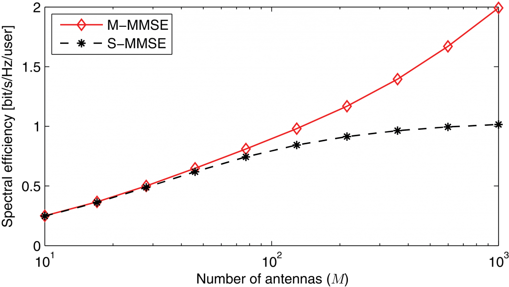
In the light of this new result, I wish that we would not have made the following remark in our 2011 Allerton paper:

“Note that a BS could theoretically estimate
all channel matrices \mathbf{H}_l (…) to further
improve the performance. Nevertheless, high path loss to
neighboring cells is likely to render these channel estimates unreliable and the potential performance gains are expected to be marginal.”

We could not have been more wrong about it!

In summary, although we did not understand the importance of M-MMSE combining in 2011, I believe that we were asking the right questions. In particular, the consideration of individual channel covariance matrices for each UE has been an important step for the analysis of Massive MIMO systems. A key lesson that I have learned from this story for my own research is that one should always question fundamental assumptions and wisdom.

Massive MIMO at 60 GHz vs. 2 GHz: How Many More Antennas?

The Brooklyn summit last week was a great event. I gave a talk (here are the slides) comparing MIMO at “PCS” (2 GHz) and mmWave (60 GHz) in line-of-sight. There are two punchlines: first, scientifically, while a link budget calculation might predict that 128.000 mmWave antennas are needed to match up the performance of 128-antenna PCS MIMO, there is a countervailing effect in that increasing the number of antennas improves channel orthogonality so that only 10.000 antennas are required. Second, practically, although 10.000 is a lot less than 128.000, it is still a very large number! Here is a writeup with some more detail on the comparison.

I also touched the (for sub-5 GHz bands somewhat controversial) topic of hybrid beamforming, and whether that would reduce the required amount of hardware.

A question from the audience was whether the use of antennas with larger physical aperture (i.e., intrinsic directivity) would change the conclusions. The answer is no: the use of directional antennas is more or less equivalent to sectorization. The problem is that to exploit the intrinsic gain, the antennas must a priori point “in the right direction”. Hence, in the array, only a subset of the antennas will be useful when serving a particular terminal. This impacts both the channel gain (reduced effective aperture) and orthogonality (see, e.g, Figure 7.5 in this book).

There was also a stimulating panel discussion afterwards. One question discussed in the panel concerned the necessity, or desirability, of using multiple terminal antennas at mmWave. Looking only at the link budget, base station antennas could be traded against terminal antennas – however, that argument neglects the inevitably lost orthogonality, and furthermore it is not obvious how beam-finding/tracking algorithms will perform (millisecond coherence time at pedestrian speeds!). Also, obviously, the comparison I presented is extremely simplistic – to begin with, the line-of-sight scenario is extremely favorable for mmWaves (blocking problems), but also, I entirely neglected polarization losses. Solely any attempts to compensate for these problems are likely to require multiple terminal antennas.

Other topics touched in the panel were the viability of Massive MIMO implementations. Perhaps the most important comment in this context made was by Ian Wong of National Instruments: “In the past year, we’ve actually shown that [massive MIMO] works in reality … To me, the biggest development is that the skeptics are being quiet.” (Read more about that here.)

Reproducible Massive MIMO Research

Reproducibility is fundamental to scientific research. If you develop a new algorithm and use simulations/experiments to claim its superiority over prior algorithms, your claims are only credible if other researchers can reproduce and confirm them.

The first step towards reproducibility is to describe the simulation procedure in such detail that another researcher can repeat the simulation, but a major effort is typically needed to reimplement everything. The second step is to make the simulation code publicly available, so that any scientist can review it and easily reproduce the results. While the first step is mandatory for publishing a scientific study, there is a movement towards open science that would make also the second step a common practice.

I understand that some researchers are skeptical towards sharing their simulation code, in fear of losing their competitive advantage towards other research groups. My personal principle is to not share any code until the research study is finished and the results have been accepted for publication in a full-length journal. After that, I think that the society benefits the most if other researcher can focus on improving my and others’ research, instead of spending excessive amount of time on reimplementing known algorithms. I also believe that the primary competitive advantage in research is the know-how and technical insights, while the simulation code is of secondary importance.

On my GitHub page, I have published Matlab code packages that reproduces the simulation results in one book, one book chapter, and more than 15 peer-reviewed articles. Most of these publications are related to MIMO or Massive MIMO. I see many benefits from doing this:

1) It increases the credibility of my research group’s work;

2) I write better code when I know that other people will read it;

3) Other researchers can dedicate their time into developing new improved algorithms and compare them with my baseline implementations;

4) Young scientists may learn how to implement a basic simulation environment by reading the code.

I hope that other Massive MIMO researchers will also make their simulation code publicly available. Maybe you have already done that? In that case, please feel free to write a comment to this post with a link to your code.

Book Review: The 5G Myth

The 5G Myth is the provocative title of a recent book by William Webb, CEO of Weightless SIG, a standard body for IoT/M2M technology. In this book, the author tells a compelling story of a stagnating market for cellular communications, where the customers are generally satisfied with the data rates delivered by the 4G networks. The revenue growth for the mobile network operators (MNOs) is relatively low and also in decay, since the current services are so good that the customers are unwilling to pay more for improved service quality. Although many new wireless services have materialized over the past decade (e.g., video streaming, social networks, video calls, mobile payment, and location-based services), the MNOs have failed to take the leading role in any of them. Instead, the customers make use of external services (e.g., Youtube, Facebook, Skype, Apple Pay, and Google Maps) and only pay the MNOs to deliver the data bits.

The author argues that, under these circumstances, the MNOs have little to gain from investing in 5G technology. Most customers are not asking for any of the envisaged 5G services and will not be inclined to pay extra for them. Webb even compares the situation with the prisoner’s dilemma: the MNOs would benefit the most from not investing in 5G, but they will anyway make investments to avoid a situation where customers switch to a competitor that has invested in 5G. The picture that Webb paints of 5G is rather pessimistic compared to a recent McKinsey report, where the more cost-efficient network operation is described as a key reason for MNOs to invest in 5G.

The author provides a refreshing description of the market for cellular communications, which is important in a time when the research community focuses more on broad 5G visions than on the customers’ actual needs. The book is thus a recommended read for 5G researchers, since we should all ask ourselves if we are developing a technology that tackles the right unsolved problems.

Webb does not only criticize the economic incentives for 5G deployment, but also the 5G visions and technologies in general. The claims are in many cases reasonable; for example, Webb accurately points out that most of the 5G performance goals are overly optimistic and probably only required by a tiny fraction of the user base. He also accurately points out that some “5G applications” already have a wireless solution (e.g., indoor IoT devices connected over WiFi) or should preferably be wired (e.g., ultra-reliable low-latency applications such as remote surgery).

However, it is also in this part of the book that the argumentation sometimes falls short. For example, Webb extrapolates a recent drop in traffic growth to claim that the global traffic volume will reach a plateau in 2027. It is plausible that the traffic growth rate will reduce as a larger and larger fraction of the global population gets access to wireless high-speed connections. But one should bear in mind that we have witnessed an exponential growth in wireless communication traffic for the past century (known as Cooper’s law), so this trend can just as well continue for a few more decades, potentially at a lower growth rate than in the past decade.

Webb also provides a misleading description of multiuser MIMO by claiming that 1) the antenna arrays would be unreasonable large at cellular frequencies and 2) the beamforming requires complicated angular beam-steering. These are two of the myths that we dispelled in the paper “Massive MIMO: Ten myths and one grand question” last year. In fact, testbeds have demonstrated that massive multiuser MIMO is feasible in lower frequency bands, and particularly useful to improve the spectral efficiency through coherent beamforming and spatial multiplexing of users. Reciprocity-based beamforming is a solution for mobile and cell-edge users, for which angular beam-steering indeed is inefficient.

The book is not as pessimistic about the future as it might seem from this review. Webb provides an alternative vision for future wireless communications, where consistent connectivity rather than higher peak rates is the main focus. This coincides with one of the 5G performance goals (i.e., 50 Mbit/s everywhere), but Webb advocates an extensive government-supported deployment of WiFi instead of 5G technology. The use WiFi is not a bad idea; I personally consume relatively little cellular data since WiFi is available at home, at work, and at many public locations in Sweden. However, the cellular services are necessary to realize the dream of consistent connectivity, particularly outdoors and when in motion. This is where a 5G cellular technology that delivers better coverage and higher data rates at the cell edge is highly desirable. Reciprocity-based Massive MIMO seems to be the solution that can deliver this, thus Webb would have had a stronger case if this technology was properly integrated into his vision.

In summary, the combination of 5G Massive MIMO for wide-area coverage and WiFi for local-area coverage might be the way to truly deliver consistent connectivity.

Real-Time Massive MIMO DSP at 50 milliWatt

Colleagues at Lund University presented last month a working circuit that performs, in real time, zero-forcing decoding and precoding of 8 simultaneous terminals with 128 base station antennas, over a 20 MHz bandwidth at a power consumption of about 50 milliWatt.

Impressive, and important.

Granted, this number does not include the complexity of FFTs, sampling rate conversions, and several other (non-insignificant) tasks; however, it does include the bulk of the “Massive-MIMO”-specific digital processing. The design exploits a number of tricks and Massive-MIMO specific properties: diagonal dominance of the channel Gramian, in particular, in sufficiently favorable propagation.

When I started work on Massive MIMO in 2009, the common view held was that the technology would be infeasible because of computational complexity. Particularly, the sheer idea of performing zero-forcing processing in real time was met with, if not ridicule, extreme skepticism. We quickly realized, however, that a reasonable DSP implementation would require no more than some ten Watt. While that is a small number in itself, it turned out to be an overestimate by orders of magnitude!

I spoke with some of the lead inventors of the chip, to learn more about its design. First, the architectures for decoding and for precoding differ a bit. While there is no fundamental reason for why this has to be so, one motivation is the possible use of nonlinear detectors on uplink. (The need for such detectors, for most “typical” cellular Massive MIMO deployments, is not clear – but that is another story.)

Second, and more importantly, the scalability of the design is not clear. While the complexity of the matrix operations themselves scale fast with the dimension, the precision in the arithmetics may have to be increased as well – resulting in a much-faster-than-cubically overall complexity scaling. Since Massive MIMO operates at its best when multiplexing to many tens of terminals (or even thousands, in some applications), significant challenges remain for the future. That is good news for circuit engineers, algorithm designers, and communications theoreticians alike. The next ten years will be exciting.

News – commentary – mythbusting