Pilots are predefined reference signals that are transmitted to let the receiver estimate the channel. While many communication systems have pilot transmissions in both uplink and downlink, the canonical communication protocol in Massive MIMO only contains uplink pilots. In this blog post, I will explain when downlink pilots are needed and why we can omit them in Massive MIMO.
Consider the communication link between a single-antenna user and an  -antenna base station (BS). The channel vector
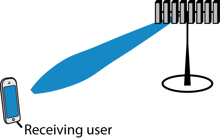
  varies over time and frequency in a way that is often modeled as random fading. In each channel coherence blocks, the BS selects a precoding vector
  and uses it for downlink transmission. The precoding reduces the multiantenna vector channel to an effective single-antenna scalar channel

The receiving user does not need to know the full -dimensional vectors  and
and  . However, to decode the downlink data in a successful way, it needs to learn the complex scalar channel
  . The difficulty in learning depends strongly on the mechanism of precoding selection. Two examples are considered below.
Codebook-based precoding
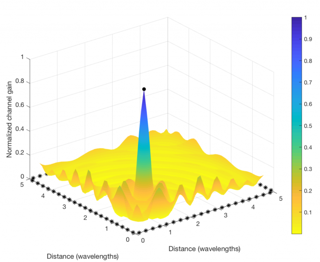
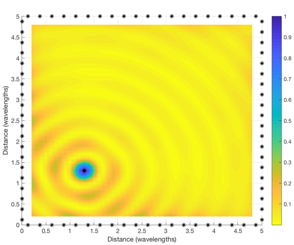
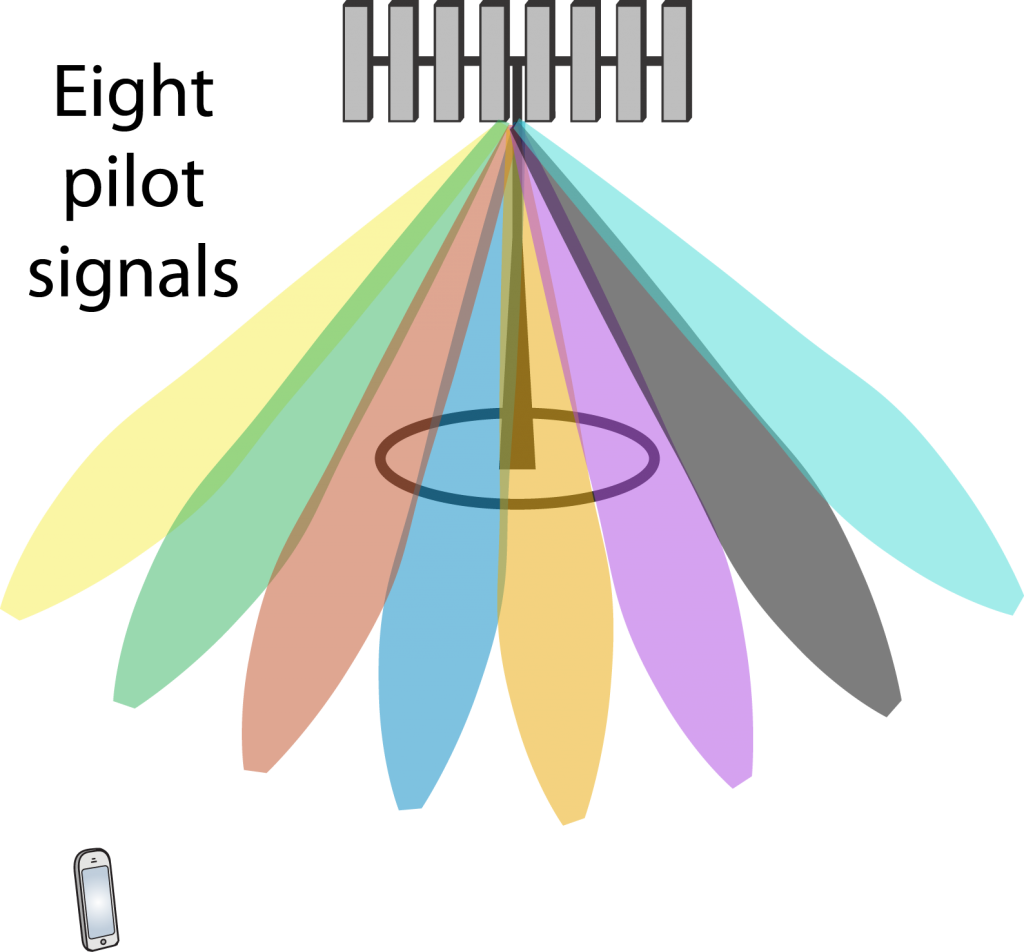 In this case, the BS tries out a set of different precoding vectors from a codebook (e.g., a grid of beams, as shown to the right) by sending one downlink pilot signal through each one of them. The user measures for each one of them and feeds back the index of the one that maximizes the channel gain
  . The BS will then transmit data using that precoding vector. During the data transmission,
  can have any phase, but the user already knows the phase and can compensate for it in the decoding algorithm.
If multiple users are spatially multiplexed in the downlink, the BS might use another precoding vector than the one selected by the user. For example, regularized zero-forcing might be used to suppress interference. In that case, the magnitude of the channel changes, but the phase remains the same. If phase-shift keying (PSK) is used for communication, such that no information is encoded in the signal amplitude, no estimation of is needed for decoding (but it can help to reduce the error probability). If quadrature amplitude modulation (QAM) is used instead, the user needs to learn also to decode the data. The unknown magnitude can be estimated blindly based on the received signals. Hence, no further pilot transmission is needed.
Reciprocity-based precoding
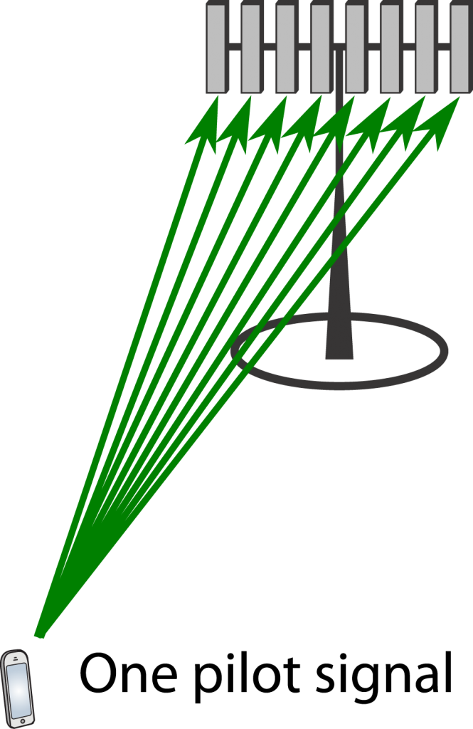 In this case, the user transmits a pilot signal in the uplink, which enables the BS to directly estimate the entire channel vector . For the sake of argument, suppose this estimation is perfect and that maximum ratio transmission with
  is used for downlink data transmission. The effective channel gain will then be

which is a positive scalar. Hence, the user only needs to learn the magnitude of because the phase is always zero. Estimation of can be implemented without downlink pilots, either by relying on channel hardening or by blind estimation based on the received signals. The former only works well in Massive MIMO with very many antennas, while the latter can be done in any system (including codebook-based precoding).
Conclusion
We generally need to compensate for the channel’s phase-shift at some place in a wireless system. In codebook-based precoding, the compensation is done at the user-side, based on the received signals from the downlink pilots. This is the main approach in 4G systems, which is why downlink pilots are so commonly used. In contrast, when using reciprocity-based precoding, the phase-shifts are compensated for at the BS-side using the uplink pilots. In either case, explicit pilot signals are only needed in one direction: uplink or downlink. If the estimation is imperfect, there will be some remaining phase ambiguity, which can be estimated blindly since we know that it is small (i.e., of all possible phase-rotations that could have resulted in the received signal, the smallest one is most likely).
When we have access to TDD spectrum, we can choose between the two precoding methods mentioned above. The reciprocity-based approach is preferable in terms of less overhead signaling; one pilot per user instead of one per index in the codebook (the codebook size needs to grow with the number of antennas), and no feedback is needed. That is why this approach is taken in the canonical form of Massive MIMO.


 -antenna base station (BS) serves
  single-antenna users. The large-scale channel gains include pathloss with exponent
  and shadowing having log-scale standard deviation
  , with the gain between the
  th BS and the
  th user served by a BS of interest denoted by
  .
.
 is the gain from the serving BS and
  is the share of that BS’s power allocated to user
  .
. , with the proportionality constant ensuring that
  . This makes
  . Moreover, as
 , which makes it valid for arbitrary BS locations.
 . Define
  as the solution to
  where
where  is the lower incomplete gamma function. For
  , in particular,
  . Under a uniform power allocation, the CDF of
  is available in an explicit form involving the Gauss hypergeometric function
  (available in MATLAB and Mathematica):
 ” indicates asymptotic (
 ) equality,
  is such that the CDF is continuous, and
 :
:

 with CDF
  readily characterizable from the expressions given earlier. From
  , the sum spectral efficiency at the BS of interest can be found as
  Expressions for the averages
 ![\bar{C} = \mathbb{E} \big[ C_k \big]](https://ma-mimo.ellintech.se/wp-content/ql-cache/quicklatex.com-a887caab28778e8d91a237bcc86a9f3e_l3.png "Rendered by QuickLaTeX.com") and
and ![\bar{C}_{\scriptscriptstyle \Sigma} = \mathbb{E} \! \left[ C_{\scriptscriptstyle \Sigma} \right]](https://ma-mimo.ellintech.se/wp-content/ql-cache/quicklatex.com-865de5351a43ee6f0405ddb531ed84ee_l3.png "Rendered by QuickLaTeX.com") are further available in the form of single integrals.
are further available in the form of single integrals.
 . For the special case of

 ,
,  and
and  –
– dB with the analysis. The behaviors with these typical outdoor values of
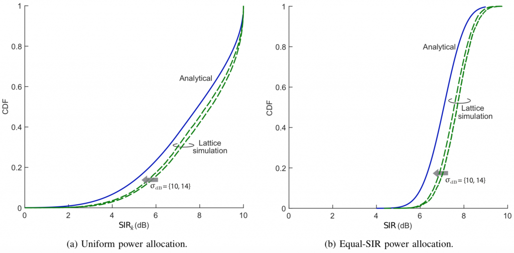
 and
and  . Figs. 2a-2b compare the simulations for
  dB with the analysis, and the agreement is now complete. The simulated average spectral efficiency with a uniform power allocation is
  b/s/Hz/user while (2) gives
  b/s/Hz/user.
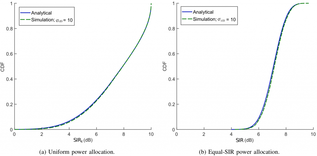
 –
– with very conservative premises) where these effects are rather minor, and the analysis is hence applicable.