Our 2014 massive MIMO tutorial paper won the IEEE ComSoc best tutorial paper award this year. The idea when writing that paper was to summarize the state of the technology, and to point out research directions that were relevant (at that time). It is of course, reassuring to see that many of those research directions evolved into entire sub-fields themselves in our community. Naturally, in the envisioning of these directions I also made some speculations.
It looks to me now that two of these speculations were wrong:
First, “Massive MIMO increases the robustness against both unintended man-made interference and intentional jamming.” This is only true with some qualifiers, or possibly not true at all. (Actually I don’t really know, and I don’t think it is known for sure. It seems that this question remains a rather pertinent research direction for anyone interested in physical layer security and MIMO.) Subsequent research by others showed that Massive MIMO can be extraordinarily susceptible to attacks on the pilot channels, revealing an important, fundamental vulnerability at least if standard pilot-based channel estimation is used and no excess dimensions are “wasted” on interference suppression or detection. Basically this pilot channel attack exploits the so-called pilot contamination phenomenon, “hijacking” the reciprocity-based beamforming mechanism.
Second, “In a way, massive MIMO relies on the law of large numbers to make sure that noise, fading, and hardware imperfections average out when signals from a large number of antennas are combined in the air.” This is not generally true, except for in-band distortion and with many simultaneously multiplexed users and frequency selective Rayleigh fading. In general the distortion that results from hardware imperfections is correlated among the antennas. In the special case of line-of-sight with a single terminal, an important basic reference case, the distortion is identical (up to a phase shift) at all antennas, hence resulting in a rank-one transmission: the distortion is beamformed in the same direction as the signal of interest and hardware imperfections do not “average out” at all.
This is particularly serious for out-band effects. Readers interested in a thorough mathematical treatment may consult my student’s recent Ph.D. dissertation.
Have you found any more? Let me know. The knowledge in the field continues to evolve.
This is supposedly a simple question to answer; an antenna is a device that emits radio waves. However, it is easy to get confused when comparing wireless communication systems with different number of transmit antennas, because these systems might use antennas with different physical sizes and properties. In fact, you can seldom find fair comparisons between contemporary single-antenna systems and Massive MIMO in the research literature.
Each antenna type has a predefined radiation pattern, which describes its inherent directivity; that is, how the gain of the emitted signal differs in different angular directions. An ideal isotropic antenna has no directivity, but a practical antenna always has a certain directivity, measured in dBi. For example, a half-wavelength dipole antenna has 2.15 dBi, which means that there is one angular direction in which the emitted signal is 2.15 dB stronger than it would be with a corresponding isotropic antenna. On the other hand, there are other angular directions in which the emitted signal is weaker. This is not a problem as long as there will not be any receivers in those directions.
In cellular communications, we are used to deploying large vertical antenna panels that cover a 120 degree horizontal sector and have a strong directivity of 15 dBi or more. Such a panel is made up of many small radiating elements, each having a directivity of a few dBi. By feeding them with the same input signal, a higher dBi is achieved for the panel. For example, if the panel consists of 8 patch antenna elements, each having 7 dBi, then you get a 7+10·log10(8) = 16 dBi antenna.
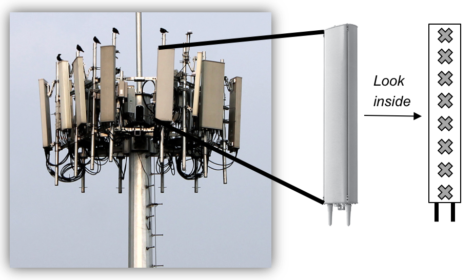
Figure 1: Photo of an LTE site with three 8TX-sectors.
The picture above shows a real LTE site that I found in Nanjing, China, a couple of years ago. Looking at it from above, the site is structured as illustrated to the right. The site consists of three sectors, each containing a base station with four vertical panels. If you would look inside one of the panels, you will (probably) find 8 cross-polarized vertically stacked radiating elements, as illustrated in Figure 1. There are two RF input signals per panel, one per polarization, thus each panel acts as two antennas. This is how LTE with 8TX-sectors is deployed: 4 panels with dual polarization per base station.
At the exemplified LTE site, there is a total of 8·8·3 =192 radiating elements, but only 8·3 = 24 antennas. This disparity can lead to a lot of confusion. The Massive MIMO version of the exemplified LTE site may have the same form factor, but instead of 24 antennas with 16 dBi, you would have 192 antennas with 7 dBi. More precisely, you would connect each of the existing radiating elements to a separate RF input signal to create a larger number of antennas. Therefore, I suggest to use the following antenna definition from the book Massive MIMO Networks:
Definition: An antenna consists of one or more radiating elements (e.g., dipoles) which are fed by the same RF signal. An antenna array is composed of multiple antennas with individual RF chains.
Note that, with this definition, an array that uses analog beamforming (e.g., a phased array) only constitutes one antenna. It is usually called an adaptive antenna since the radiation pattern can be changed over time, but it is nevertheless a single antenna. Massive MIMO for sub-6 GHz frequencies is all about adding RF chains (also known as antenna ports), while not necessarily adding more radiating elements than in a contemporary system.
What is the purpose of having more RF chains?
With more RF chains, you have more degrees of freedom to modify the radiation pattern of the transmitted signal based on where the receiver is located. When transmitting a precoded signal to a single user, you adjust the phases of the RF input signals to make them all combine constructively at the intended receiver.
The maximum antenna/array gain is the same when using one 16 dBi antenna and when using 8 antennas with 7 dBi. In the first case, the radiation pattern is usually static and thus only a line-of-sight user located in the center of the cell sector will obtain this gain. However, if the antenna is adaptive (i.e., supports analog beamforming), the main lobe of the radiation pattern can be also steered towards line-of-sight users located in other angular directions. This feature might be sufficient for supporting the intended single-user use-cases of mm-wave technology (see Figure 4 in this paper).
In contrast, in the second case, we can adjust the radiation pattern by 8-antenna precoding to deliver the maximum gain to any user in the sector. This feature is particularly important for non-line-of-sight users (e.g., indoor use-cases), for which the signals from the different radiating elements will likely be received with “random” phase shifts and therefore add non-constructively, unless we compensate for the phases by digital precoding.
Note that most papers on Massive MIMO keep the antenna gain constant when comparing systems with different number of antennas. There is nothing wrong with doing that, but one cannot interpret the single-antenna case in such a study as a contemporary system.
Another, perhaps more important, feature of having multiple RF chains is that we can spatially multiplex several users when having multiple antennas. For this you need at least as many RF inputs as there are users. Each of them can get the full array gain and the digital precoding can be also used to avoid inter-user interference.
Last year, I wrote a post about channel hardening. To recap, the achievable data rate of a conventional single-antenna channel varies rapidly over time due to the random small-scale fading realizations, and also over frequency due to frequency-selective fading. However, when you have many antennas at the base station and use them for coherent precoding/combining, the fluctuations in data rate average out; we then say that the channel hardens. One follow-up question that I’ve got several times is:
Can we utilize the channel hardening to estimate the channels less frequently?
Unfortunately, the answer is no. Whenever you move approximately half a wavelength, the multi-path propagation will change each element of the channel vector. The time it takes to move such a distance is called a coherence time. This time is the same irrespectively of how many antennas the base station has and, therefore, you still need to estimate the channel once per coherence time. The same applies to the frequency domain, where the coherence bandwidth is determined by the propagation environment and not the number of antennas.
The following flow-chart shows what need to happen in every channel coherence time:
When you get a new realization (at the top of the flow-chart), you compute an estimate (e.g., based on uplink pilots), then you use the estimate to compute a new receive combining vector and transmit precoding vector. It is when you have applied these vectors to the channel that the hardening phenomena appears; that is, the randomness averages out. If you use maximum ratio (MR) processing, then the random realization h1 of the channel vector turns into an almost deterministic scalar channel ||h1||2. You can communicate over the hardened channel with gain ||h1||2 until the end of the coherence time. You then start over again by estimating the new channel realization h2, applying MR precoding/combining again, and then you get ||h2||2 ≈ ||h1||2.
In conclusion, channel hardening appears after coherent combining/precoding has been applied. To maintain a hardened channel over time (and frequency), you need to estimate and update the combining/precoding as often as you would do for a single-antenna channel. If you don’t do that, you will gradually lose the array gain until the point where the channel and the combining/precoding are practically uncorrelated, so there is no array gain left. Hence, there is more to lose from estimating channels too infrequently in Massive MIMO systems than in conventional systems. This is shown in Fig. 10 in a recent measurement paper from Lund University, where you see how the array gain vanishes with time. However, the Massive MIMO system will never be worse than the corresponding single-antenna system.
The signal-to-noise ratio (SNR) generally depends on the transmit power, channel gain, and noise power:
Since the spectral efficiency (bit/s/Hz) and many other performance metrics of interest depend on the SNR, and not the individual values of the three parameters, it is a common practice to normalize one or two of the parameters to unity. This habit makes it easier to interpret performance expressions, to select reasonable SNR ranges, and to avoid mistakes in analytical derivations.
There are, however, situations when the absolute value of the transmitted/received signal power matters, and not the relative value with respect to the noise power, as measured by the SNR. In these situations, it is easy to make mistakes if you use normalized parameters. I see this type of errors far too often, both as a reviewer and in published papers. I will give some specific examples below, but I won’t tell you who has made these mistakes, to not point the finger at anyone specifically.
Wireless energy transfer
Electromagnetic radiation can be used to transfer energy to wireless receivers. In such wireless energy transfer, it is the received signal energy that is harvested by the receiver, not the SNR. Since the noise power is extremely small, the SNR is (at least) a billion times larger than the received signal power. Hence, a normalization error can lead to crazy conclusions, such as being able to transfer energy at a rate of 1 W instead of 1 nW. The former is enough to keep a wireless transceiver on continuously, while the latter requires you to harvest energy for a long time period before you can turn the transceiver on for a brief moment.
Energy efficiency
The energy efficiency (EE) of a wireless transmission is measured in bit/Joule. The EE is computed as the ratio between the data rate (bit/s) and the power consumption (Watt=Joule/s). While the data rate depends on the SNR, the power consumption does not. The same SNR value can be achieved over a long propagation distance by using high transmit power or over a short distance by using a low transmit power. The EE will be widely different in these cases. If a “normalized transmit power” is used instead of the actual transmit power when computing the EE, one can get EEs that are one million times smaller than they should be. As a rule-of-thumb, if you compute things correctly, you will get EE numbers in the range of 10 kbit/Joule to 10 Mbit/Joule.
Noise power depends on the bandwidth
The noise power is proportional to the communication bandwidth. When working with a normalized noise power, it is easy to forget that a given SNR value only applies for one particular value of the bandwidth.
Some papers normalize the noise variance and channel gain, but then make the SNR equal to the unnormalized transmit power (measured in W). This may greatly overestimate the SNR, but the achievable rates might still be in the reasonable range if you operate the system in an interference-limited regime.
Some papers contain an alternative EE definition where the spectral efficiency (bit/s/Hz) is divided by the power consumption (Joule/s). This leads to the alternative EE unit bit/Joule/Hz. This definition is not formally wrong, but gives the misleading impression that one can multiply the EE value with any choice of bandwidth to get the desired number of bit/Joule. That is not the case since the SNR only holds for one particular value of the bandwidth.
Knowing when to normalize
In summary, even if it is convenient to normalize system parameters in wireless communications, you should only do it if you understand when normalization is possible and when it is not. Otherwise, you can make embarrassing mistakes, such as submitting a paper where the results are six orders of magnitude wrong. And, unfortunately, there are several such papers that have been published and these create a bad circle by tricking others into making the same mistakes.
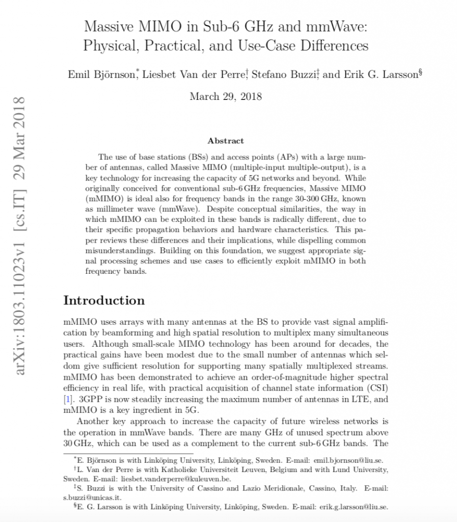
One of the most read posts on this blog is Six differences between Massive MIMO for sub-6 GHz and mmWave, where we briefly outlined the key differences between how the Massive MIMO technology would be implemented and utilized in different frequency bands. Motivated by the great feedback and interest in this topic, we joined forces with Liesbet Van der Perre and Stefano Buzzi to write a full-length magazine article. It has recently been submitted to IEEE Wireless Communications and a pre-print can be found on ArXiv.org:
The hardback version of the massive new bookMassive MIMO Networks: Spectral, Energy, and Hardware Efficiency (by Björnson, Sanguinetti, Hoydis) is currently available for the special price of $70 (including worldwide shipping). The original price is $99.
This price is available until the end of April when buying the book directly from the publisher through the following link:
Note: The book’s authors will give a joint tutorial on April 15 at WCNC 2018. A limited number of copies of the book will be available for sale at the conference and if you attend the tutorial, you will receive even better deal on buying the book!
While the research literature is full of papers that design wireless communication systems under constraints on the maximum transmitted power, in practice, it might be constraints on the equivalent isotropically radiated power (EIRP) or the out-of-band radiation that limit the system operation.

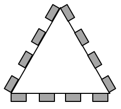 The picture above shows a real LTE site that I found in Nanjing, China, a couple of years ago. Looking at it from above, the site is structured as illustrated to the right. The site consists of three sectors, each containing a base station with four vertical panels. If you would look inside one of the panels, you will (probably) find 8 cross-polarized vertically stacked radiating elements, as illustrated in Figure 1. There are two RF input signals per panel, one per polarization, thus each panel acts as two antennas. This is how LTE with 8TX-sectors is deployed: 4 panels with dual polarization per base station.
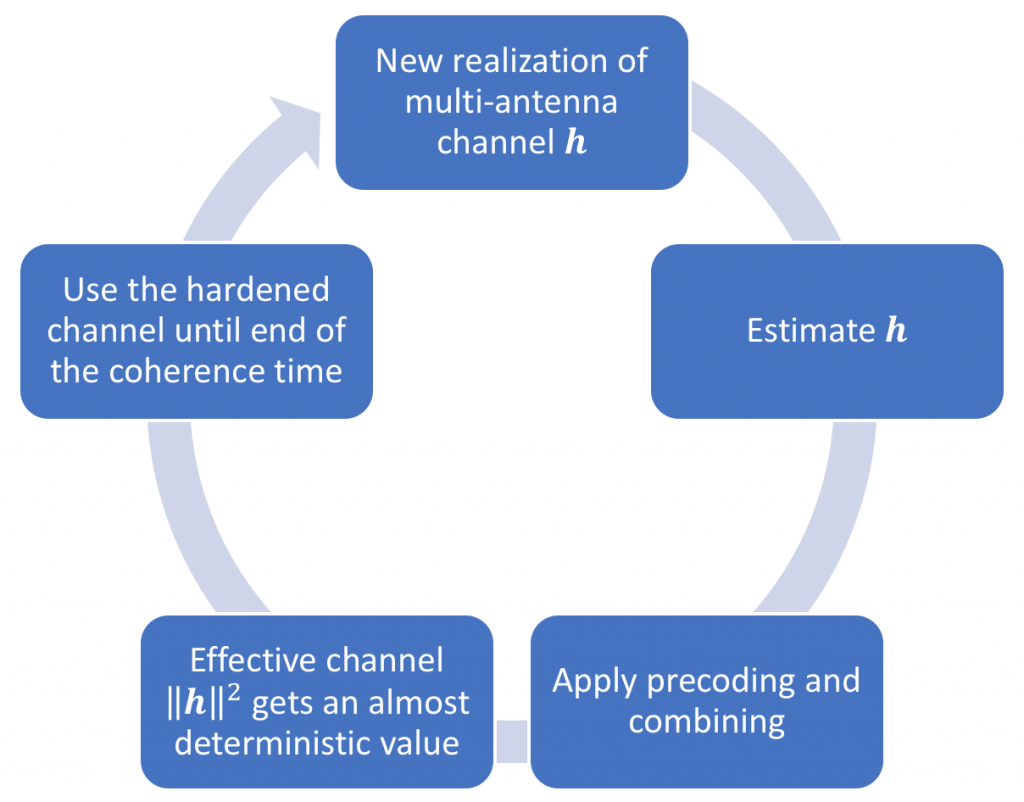

 The hardback version of the massive