

More Bandwidth Requires More Power or Antennas
The main selling point of millimeter-wave communications is the abundant bandwidth available in such frequency bands; for example, 2 GHz of bandwidth instead of 20 MHz as in conventional cellular networks. The underlying argument is that the use of much wider bandwidths immediately leads to much higher capacities, in terms of bit/s, but the reality is not that simple.
To look into this, consider a communication system operating over a bandwidth of  Hz. By assuming an additive white Gaussian noise channel, the capacity becomes

where  W is the transmit power,
  is the channel gain, and
  W/Hz is the power spectral density of the noise. The term
  inside the logarithm is referred to as the signal-to-noise ratio (SNR).
Since the bandwidth appears in front of the logarithm, it might seem that the capacity grows linearly with the bandwidth. This is not the case since also the noise term  in the SNR also grows linearly with the bandwidth. This fact is illustrated by Figure 1 below, where we consider a system that achieves an SNR of 0 dB at a reference bandwidth of 20 MHz. As we increase the bandwidth towards 2 GHz, the capacity grows only modestly. Despite the 100 times more bandwidth, the capacity only improves by
  , which is far from the
  that a linear increase would give.
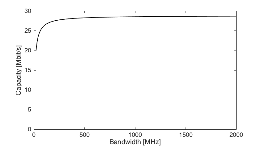
The reason for this modest capacity growth is the fact that the SNR reduces inversely proportional to the bandwidth. One can show that

The convergence to this limit is seen in Figure 1 and is relatively fast since  for
for  .
.
To achieve a linear capacity growth, we need to keep the SNR fixed as the bandwidth increases. This can be achieved by increasing the transmit power proportionally to the bandwidth, which entails using more power when operating over a wider bandwidth. This might not be desirable in practice, at least not for battery-powered devices.
An alternative is to use beamforming to improve the channel gain. In a Massive MIMO system, the effective channel gain is  , where
  is the number of antennas and
  is the gain of a single-antenna channel. Hence, we can increase the number of antennas proportionally to the bandwidth to keep the SNR fixed.
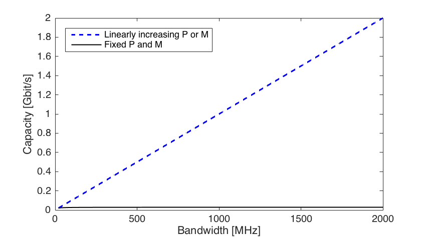
Figure 2 considers the same setup as in Figure 1, but now we also let either the transmit power or the number of antennas grow proportionally to the bandwidth. In both cases, we achieve a capacity that grows proportionally to the bandwidth, as we initially hoped for.
In conclusion, to make efficient use of more bandwidth we require more transmit power or more antennas at the transmitter and/or receiver. It is worth noting that these requirements are purely due to the increase in bandwidth. In addition, for any given bandwidth, the operation at millimeter-wave frequencies requires much more transmit power and/or more antennas (e.g., additional constant-gain antennas or one constant-aperture antenna) just to achieve the same SNR as in a system operating at conventional frequencies below 5 GHz.
Massive MIMO Trials in LTE Networks
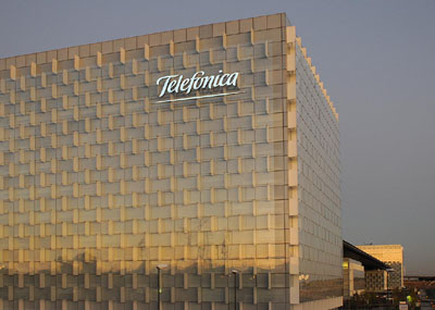
Massive MIMO is often mentioned as a key 5G technology, but could it also be exploited in currently standardized LTE networks? The ZTE-Telefónica trials that were initiated in October 2016 shows that this is indeed possible. The press release from late last year describes the first results. For example, the trial showed improvements in network capacity and cell-edge data rates of up to six times, compared to traditional LTE.
The Massive MIMO blog has talked with Javier Lorca Hernando at Telefónica to get further details. The trials were carried out at the Telefónica headquarters in Madrid. A base station with 128 antenna ports was deployed at the rooftop of one of their buildings and the users were located in one floor of the central building, approximately 100 m from the base station. The users basically had cell-edge conditions, due to the metallized glass and multiple metallic constructions surrounding them.
The uplink and downlink data transmissions were carried out in the 2.6 GHz band. Typical Massive MIMO time-division duplex (TDD) operation was considered, where the uplink detection and downlink precoding is based on uplink pilots and channel reciprocity. The existing LTE sounding reference signals (SRSs) were used as uplink pilots. The reciprocity-based precoding was implemented by using LTE’s transmission mode 8 (TM8), which supports any type of precoding. Downlink pilots were used for link adaptation and demodulation purposes.
It is great to see that Massive MIMO can be also implemented in LTE systems. In this trial, the users were static and relatively few, but it will be exciting to see if the existing LTE reference signals will also enable Massive MIMO communications for a multitude of mobile users!
Update: ZTE has carried out similar experiments in cooperation with Smartfren in Indonesia. Additional field trials are mentioned in the comments to this post.
Upside-Down World
The main track for 5G seems to be FDD for “old bands” below 3 GHz and TDD for “new bands” above 3 GHz (particularly mmWave frequencies). But physics advices us to the opposite:
- At lower frequencies, larger areas are covered, thus most connections are likely to experience non-line-of-sight propagation. Since channel coherence is large (scales inverse proportionally to the Doppler), there is room for many terminals to transmit uplink pilots from which the base station consequently can obtain CSI. Reciprocity-based beamforming in TDD operation is scalable with respect to the number of base station antennas and delivers great value.
- As the carrier frequency is increased, the coverage area shrinks; connections are more and more likely to experience line-of-sight propagation. At mmWave frequencies, all connections are either line-of-sight, or consist of a small number of reflected components. Then the channel can be parameterized with only few angular parameters; FDD operation with appropriate flavors of beam tracking may work satisfactorily. Reciprocity certainly would be desirable in this case too, but may not be necessary for the system to function.
Physics has given us the reciprocity principle. It should be exploited in wireless system design.
Channel Hardening Makes Fading Channels Behave as Deterministic
One of the main impairments in wireless communications is small-scale channel fading. This refers to random fluctuations in the channel gain, which are caused by microscopic changes in the propagation environments. The fluctuations make the channel unreliable, since occasionally the channel gain is very small and the transmitted data is then received in error.
The diversity achieved by sending a signal over multiple channels with independent realizations is key to combating small-scale fading. Spatial diversity is particularly attractive, since it can be obtained by simply having multiple antennas at the transmitter or the receiver. Suppose the probability of a bad channel gain realization is p. If we have M antennas with independent channel gains, then the risk that all of them are bad is pM. For example, with p=0.1, there is a 10% risk of getting a bad channel in a single-antenna system and a 0.000001% risk in an 8-antenna system. This shows that just a few antennas can be sufficient to greatly improve reliability.
In Massive MIMO systems, with a “massive” number of antennas at the base station, the spatial diversity also leads to something called “channel hardening”. This terminology was used already in a paper from 2004:
M. Hochwald, T. L. Marzetta, and V. Tarokh, “Multiple-antenna channel hardening and its implications for rate feedback and scheduling,” IEEE Transactions on Information Theory, vol. 50, no. 9, pp. 1893–1909, 2004.
In short, channel hardening means that a fading channel behaves as if it was a non-fading channel. The randomness is still there but its impact on the communication is negligible. In the 2004 paper, the hardening is measured by dividing the instantaneous supported data rate with the fading-averaged data rate. If the relative fluctuations are small, then the channel has hardened.
Since Massive MIMO systems contain random interference, it is usually the hardening of the channel that the desired signal propagates over that is studied. If the channel is described by a random M-dimensional vector h, then the ratio ||h||2/E{||h||2} between the instantaneous channel gain and its average is considered. If the fluctuations of the ratio are small, then there is channel hardening. With an independent Rayleigh fading channel, the variance of the ratio reduces with the number of antennas as 1/M. The intuition is that the channel fluctuations average out over the antennas. A detailed analysis is available in a recent paper.
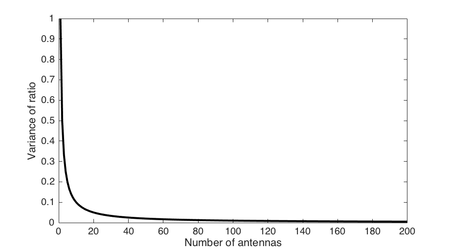
The figure above shows how the variance of ||h||2/E{||h||2} decays with the number of antennas. The convergence towards zero is gradual and so is the channel hardening effect. I personally think that you need at least M=50 to truly benefit from channel hardening.
Channel hardening has several practical implications. One is the improved reliability of having a nearly deterministic channel, which results in lower latency. Another is the lack of scheduling diversity; that is, one cannot schedule users when their ||h||2 are unusually large, since the fluctuations are small. There is also little to gain from estimating the current realization of ||h||2, since it is relatively close to its average value. This can alleviate the need for downlink pilots in Massive MIMO.
Pilot Contamination: an Ultimate Limitation?
Many misconceptions float around about the pilot contamination phenomenon. While existent in any multi-cellular system, its effect tends to be particularly pronounced in Massive MIMO due to the presence of coherent interference, that scales proportionally to the coherent beamforming gain. (Chapter 4 in Fundamentals of Massive MIMO gives the details.)
A good system design definitely must not ignore pilot interference. While it is easily removed “on the average” through greater-than-one reuse, the randomness present in wireless communications – especially the shadow fading – will occasionally cause a few terminals to be severely hit by pilot contamination and bring down their performance. This is problematic whenever we are concerned about the provision of uniformly great service in the cell – and that is one of the principal selling arguments for Massive MIMO. Notwithstanding, the impact of pilot contamination can be reduced significantly in practice by appropriate pilot reuse and judicious power control. (Chapters 5-6 in Fundamentals of Massive MIMO gives many details.)
A more fundamental question is whether pilot contamination could be entirely overcome: Does there exist an upper bound on capacity that saturates as the number of antennas, M, is increased indefinitely? Some have speculated that it cannot; much in line with known capacity upper bounds for cellular base station cooperation. While this question may be of more academic than practical interest, it has long been open except for in some trivial special cases: If the channels of two terminals lie in non-overlapping subspaces and Bayesian channel estimation is used, the channel estimates will not be contaminated; capacity grows as log(M) when M increases without bound.
A much deeper result is established in this recent paper: the subspaces of the channel covariances may overlap, yet capacity grows as log(M). Technically, a Rayleigh fading with spatial correlation is assumed, and the correlation matrices for the contaminating terminals must only be linearly independent as M goes to infinity (exact conditions in the paper). In retrospect, this is not unreasonable given the substantial a priori knowledge exploited by the Bayesian channel estimator, but I found it amazing how weak the required conditions on the correlation matrices are. It remains unclear whether the result generalizes to the case of a growing number of interferers: letting the number of antennas go to infinity and then growing the network is not the same thing as taking an “infinite” (scalable) network and increasing the number of antennas. But this paper elegantly and rigorously answers a long-standing question that has been the subject of much debate in the community – and is a recommended read for anyone interested in the fundamental limits of Massive MIMO.
Pilot Contamination in a Nutshell
One word that is tightly connected with Massive MIMO is pilot contamination. This is a phenomenon that can appear in any communication system that operates under interference, but in this post, I will describe its basic properties in Massive MIMO.
The base station wants to know the channel responses of its user terminals and these are estimated in the uplink by sending pilot signals. Each pilot signal is corrupted by inter-cell interference and noise when received at the base station. For example, consider the scenario illustrated below where two terminals are transmitting simultaneously, so that the base station receives a superposition of their signals—that is, the desired pilot signal is contaminated.
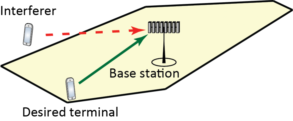
When estimating the channel from the desired terminal, the base station cannot easily separate the signals from the two terminals. This has two key implications:
First, the interfering signal acts as colored noise that reduces the channel estimation accuracy.
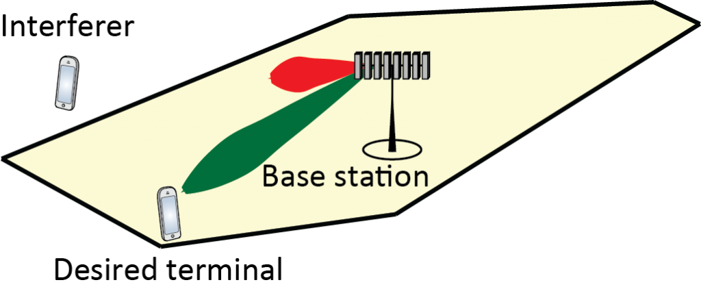
Second, the base station unintentionally estimates a superposition of the channel from the desired terminal and from the interferer. Later, the desired terminal sends payload data and the base station wishes to coherently combine the received signal, using the channel estimate. It will then unintentionally and coherently combine part of the interfering signal as well. This is particularly poisonous when the base station has M antennas, since the array gain from the receive combining increases both the signal power and the interference power proportionally to M. Similarly, when the base station transmits a beamformed downlink signal towards its terminal, it will unintentionally direct some of the signal towards to interferer. This is illustrated below.
In the academic literature, pilot contamination is often studied under the assumption that the interfering terminal sends the same pilot signal as the desired terminal, but in practice any non-orthogonal interfering signal will cause the two effects described above.