MAMMOET: Massive MIMO for Efficient Transmission

November 15, 2017 Emil Björnson Leave a comment

MAMMOET (Massive MIMO for Efficient Transmission) was the first major research project on Massive MIMO that was funded by the European Union. The project took place 2014-2016 and you might have heard about its outcomes in terms of the first demonstrations of real-time Massive MIMO that was carried out by the LuMaMi testbed at Lund University. The other partners in the project were Ericsson, Imec, Infineon, KU Leuven, Linköping University, Technikon, and Telefonica. MAMMOET was an excellent example of a collaborative project, where the telecom industry defined the system requirements and the other partners designed and evaluated new algorithms and hardware implementations to reach the requirements.

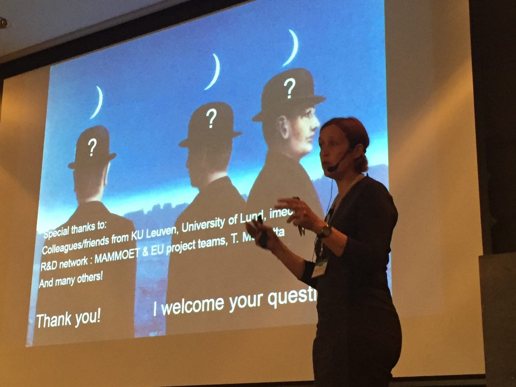
This article is an interview with Prof. Liesbet Van der Perre who was the scientific leader of the project.

Liesbet Van der Perre while disseminating results from the MAMMOET project in September 2017.

In 2012, when you began to draft the project proposal, Massive MIMO was not a popular topic. Why did you initiate the work?

– Theoretically and conceptually it seemed so interesting that it would be a pity not to work on it. The main goal of the MAMMOET project was to make conceptual progress towards a spectrally and energy efficient system and to raise the confidence level by demonstrating a practical hardware implementation. We also wanted to make channel measurements to see if they would confirm what has been seen in theory.

It seems the project partners had a clear vision from the beginning?

– It was actually very easy to write this proposal because everyone was on the same wavelength and knew what we wanted to achieve. We were all eager to start the project and learn from each other. This is quite unique and explains why the project delivered much more than promised. The fact that the team got along very well has also laid the fundament for further research collaborations.

What were the main outcomes of the project?

– We learned a lot on how things change when going from small to large arrays. New channel models are required to capture the new behaviors. We are used to that high-precision hardware is needed, but all the sudden this is not true when drastically increasing the number of antennas. You can then use low-resolution hardware and simple processing, which is very different from conventional MIMO implementation.

Some of the big conceptual differences in massive MIMO turned out to be easier to solve than expected, while some things were more problematic than foreseen. For example, it is difficult to connect all the signals together. You need to do part of the processing distributive to avoid this problem. Synchronization also turned out to be a bottleneck. If we would have known that from the start, we could have designed the testbed differently, but we thought that the channel estimation and MIMO processing would be the challenging part.

What was the most rewarding aspect of leading this project?

– The cross-fertilization of people was unique. We brought people with different background and expertise together in a room to identify the crucial problems in massive MIMO and find new solutions. For example, we realized early that interference will be a main problem and that zero-forcing processing is needed, although matched filtering was popular at the time. By carefully analyzing the zero-forcing complexity, we could show that it was almost negligible compared to other necessary processing and we later demonstrated zero-forcing in real-time at the testbed. This was surprising for many people who thought that massive MIMO would be impossible to implement since 8×8 MIMO systems are terribly complex, but many things can be simplified in massive MIMO. Looking back, it might seem that the outcomes were obvious, but these are things you don’t know until you have gone through the process.

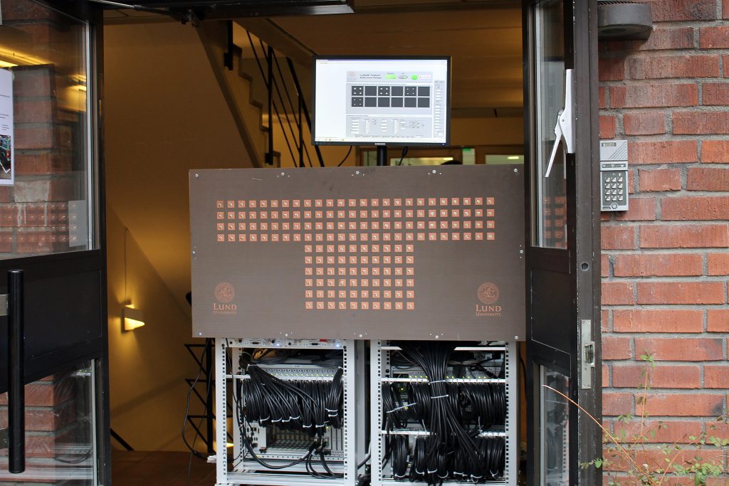
The real-time LuMaMi testbed at Lund University, the first one of its kind.

What are the big challenges that remains?

– An important challenge is how to integrate massive MIMO into a network. We assumed that there are many users and we can all give them the same time-frequency resources, but the channels and traffic are not always suitable for that. How should we decide which users to put together? We used an LTE-like frame structure, but it is important to design a frame structure that is well-suited for massive MIMO and real traffic.

There are many tradeoffs and degrees-of-freedom when designing massive MIMO systems. Would you use the technology to provide very good cell coverage or to boost small-cell capacity? Instead of delivering fiber to homes, we could use massive MIMO with very many antennas for spatial multiplexing of fixed wireless connections. Alternatively, in a mobile situation, we might not multiplex so many users. Optimizing massive MIMO for different scenarios is something that remains.

We made a lot of progress on the digital processing side in MAMMOET, while on the analog side we mainly came up with the specifications. We also did not work on the antenna design since, theoretically, it does not matter which antennas you use, but in practice it does.

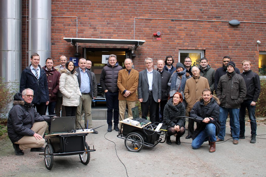
The research team of the MAMMOET project at the final review meeting of the project in February 2017.

All the deliverables and publications in the MAMMOET project can be accessed online: https://mammoet-project.technikon.com/

The deliverables contain a lot information related to use cases, requirements, channel modeling, signal processing algorithms, algorithmic implementation, and hardware implementation. Some of the results can found in the research literature, but far from everything.

Note: The author of this article worked in the MAMMOET project, but did not take part in the drafting of the proposal.

Commentary, News

Massive MIMO is Becoming a Marketing Term

November 8, 2017 Emil Björnson 3 Comments

I have been wondering for years if “MIMO” will always be a term exclusively used by engineers and a few well-informed consumers, or if it eventually becomes a word that most people are using. Will you ever hear kids saying: “I want a MIMO tablet for Christmas”?

I have been think that it can go either way – it is in the hands of marketing people. Advanced Wifi routers have been marketed with MIMO functionality for some years, but the impact is limited since most people get their routers as part of their internet subscriptions instead of buying them separately. Hence, the main question is: will handset manufactures and telecom operators start using the MIMO term when marketing products to end customers?

Maybe we have the answer because Sprint, an American telecom operator, is currently marketing their 2018 deployment of new LTE technology by talking publicly about “Massive MIMO”. As I wrote back in March, Sprint and Ericsson were to conduct field tests in the second half of 2017. Results from the tests conducted in Seattle, Washington and Plano, Texas, have now been described in a press release. The tests were carried at a carrier frequency in the 2.5 GHz band using TDD mode and an Ericsson base station with 64 transmit/receive antennas. It is fair to call this Massive MIMO, although 64 antennas is in the lower end of the interval that I would call “massive”.

The press release describes “peak speeds of more than 300 Mbps using a single 20 MHz channel”, which corresponds to a spectral efficiency of 15 bit/s/Hz. That is certainly higher than you can get in legacy LTE networks, but it is less than some previous field tests.

Hence, when the Sprint COO of Technology, Guenther Ottendorfer, describes their Massive MIMO deployment with the words “You ain’t seen nothing yet”, I hope that this means that we will see network deployments with substantially higher spectral efficiencies than 15 bit/s/Hz in the years to come.

Several videos about the field test in Seattle have recently appeared. The first one demonstrates that 100 people can simultaneously download a video, which is not possible in legacy networks. Since the base station has 64 antennas, the 100 users are probably served by a combination of spatial multiplexing and conventional orthogonal time-frequency multiplexing.

The second video provides some more technical details about the setup used in the field test.

Education, News, Technical insights

Upcoming Massive MIMO Webinars

November 7, 2017 Emil Björnson Leave a comment

IEEE ComSoc is continuing to deliver webinars on 5G topics and Massive MIMO is a key part of several of them. The format is a 40 minute presentation followed by a 20 minuter Q/A session. Hence, if you attend the webinars “live”, you have the opportunity to ask questions to the presenters. Otherwise, you can also watch each webinar afterwards. For example, 5G Massive MIMO: Achieving Spectrum Efficiency, which was given in August by Liesbet Van der Perre (KU Leuven), can still be watched.

In November, the upcoming Massive MIMO webinars are:

Massive MIMO for 5G: How Big Can it Get? by Emil Björnson (Linköping University), Thursday, 9 November 2017, 3:00 PM EST, 12:00 PM PST, 20:00 GMT.

Real-time Prototyping of Massive MIMO: From Theory to Reality by Douglas Kim (NI) and Fredrik Tufvesson (Lund University), Wednesday, 15 November 2017, 12:00 PM EST, 9:00 AM PST, 17:00 GMT.

5G, Commentary, News, Technical insights

Superimposed Pilots?

October 31, 2017 Erik G. Larsson 11 Comments

The concept of superimposed pilots is (at least 15 years) old, but clever and intriguing. The idea is to add pilot and data samples together, instead of separating them in time and/or frequency, before modulating with waveforms. More recently, the authors of this paper argued that in massive MIMO, based on certain simulations supported by asymptotic analysis, superimposed pilots provide superior performance and that there are strong reasons for superimposed pilots to make their way to practical use.

Until recently, a more rigorous analysis was unavailable. Some weeks ago the authors of this paper argued, that all things considered, the use of superimposed pilots does not offer any appreciable gains for practically interesting use cases. The analysis was based on a capacity-bounding approach for finite numbers of antennas and finite channel coherence, but it assumed the most basic form of signal processing for detection and decoding.

There still remains some hope of seeing improvements, by implementing more advanced signal processing, like zero-forcing, multicell MMSE decoding, or iterative decoding algorithms, perhaps involving “turbo” information exchange between the demodulator, channel estimation, and detector. It will be interesting to follow future work by these two groups of authors to understand how large improvements (if any) superimposed pilots eventually can give.

There are, at least, two general lessons to learn here. First, that performance predictions based on asymptotics can be misleading in practically relevant cases. (I have discussed this issue before.) The best way to perform analysis is to use rigorous capacity lower bounds, or possibly, in isolated cases of interest, link-level simulations with channel coding (for which, as it turns out, capacity bounds are a very good proxy). Second, more concretely, that while it may be tempting, to superimpose-squeeze multiple symbols into the same time-frequency-space resource, once all sources of impairments (channel estimation errors, interference) are accurately accounted for, the gains tend to evaporate. (It is for the same reason that NOMA offers no substantial gains in MIMO systems – a topic that I may return to at a later time.)

5G, Commentary, Technical insights

Six Differences Between MU-MIMO and Massive MIMO

October 17, 2017 Emil Björnson 22 Comments

Multi-user MIMO (MU-MIMO) is not a new technology, but the basic concept of using multi-antenna base stations (BSs) to serve a multitude of users has been around since the late 1980s.

An example of how MU-MIMO was illustrated prior to Massive MIMO.

I sometimes get the question “Isn’t Massive MIMO just MU-MIMO with more antennas?” My answer is no, because the key benefit of Massive MIMO over conventional MU-MIMO is not only about the number of antennas. Marzetta’s Massive MIMO concept is the way to deliver the theoretical gains of MU-MIMO under practical circumstances. To achieve this goal, we need to acquire accurate channel state information, which in general can only be done by exploiting uplink pilots and channel reciprocity in TDD mode. Thanks to the channel hardening and favorable propagation phenomena, one can also simplify the system operation in Massive MIMO.

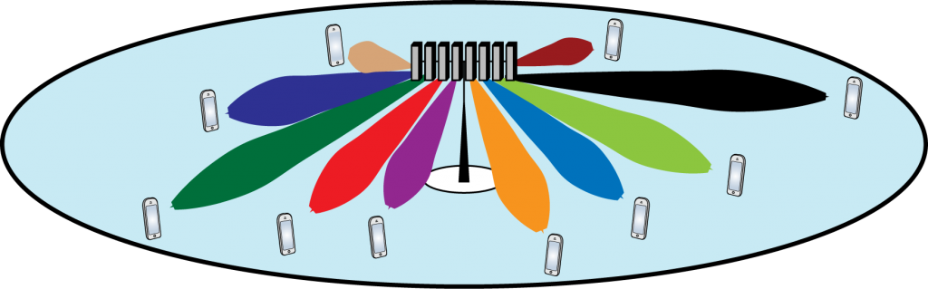
This is how Massive MIMO is often illustrated for line-of-sight operation.

Six key differences between conventional MU-MIMO and Massive MIMO are provided below.

	Conventional MU-MIMO	Massive MIMO
Relation between number of BS antennas (M) and users (K)	M ≈ K and both are small (e.g., below 10)	M ≫ K and both can be large (e.g., M=100 and K=20).
Duplexing mode	Designed to work with both TDD and FDD operation	Designed for TDD operation to exploit channel reciprocity
Channel acquisition	Mainly based on codebooks with set of predefined angular beams	Based on sending uplink pilots and exploiting channel reciprocity
Link quality after precoding/combining	Varies over time and frequency, due to frequency-selective and small-scale fading	Almost no variations over time and frequency, thanks to channel hardening
Resource allocation	The allocation must change rapidly to account for channel quality variations	The allocation can be planned in advance since the channel quality varies slowly
Cell-edge performance	Only good if the BSs cooperate	Cell-edge SNR increases proportionally to the number of antennas, without causing more inter-cell interference

Footnote: TDD stands for time-division duplex and FDD stands for frequency-division duplex.

Commentary, Education

Some Impactful Rejected Papers

October 10, 2017 Erik G. Larsson 1 Comment

Yes, my group had its share of rejected papers as well. Here are some that I specially remember:

Massive MIMO: 10 myths and one critical question. The first version was rejected by the IEEE Signal Processing Magazine. The main comment was that nobody would think that the points that we had phrased as myths were true. But in reality, each one of the myths was based on an actual misconception heard in public discussions! The paper was eventually published in the IEEE Communications Magazine instead in 2016, and has been cited more than 180 times.
Massive MIMO with 1-bit ADCs. This paper was rejected by the IEEE Transactions on Wireless Communications. By no means a perfect paper… but the review comments were mostly nonsensical. The editor stated: “The concept as such is straightforward and the conceptual novelty of the manuscript is in that sense limited.” The other authors left my group shortly after the paper was written. I did not predict the hype on 1-bit ADCs for MIMO that would ensue (and this happened despite the fact that yes, the concept as such is straightforward and its conceptual novelty is rather limited!). Hence I didn’t prioritize a rewrite and resubmission. The paper was never published, but we put the rejected manuscript on arXiv in 2014, and it has been cited 80 times.
Finally, a paper that was almost rejected upon its initial submission: Energy and Spectral Efficiency of Very Large Multiuser MIMO Systems, eventually published in the IEEE Transactions on Communications in 2013. The review comments included obvious nonsense, such as “Overall, there is not much difference in theory compared to what was studied in the area of MIMO for the last ten years.” The paper subsequently won the IEEE ComSoc Stephen O. Rice Prize, and has more than 1300 citations.

There are several lessons to learn here. First, that peer review may be the best system we know, but it isn’t perfect: disturbingly, it is often affected by incompetence and bias. Second, notwithstanding the first, that many paper rejections are probably also grounded in genuine misunderstandings: writing well takes a lot of experience, and a lot of hard, dedicated work. Finally, and perhaps most significantly, that persistence is really an essential component of success.

Commentary, Education, Technical insights

What is the Difference Between Beamforming and Precoding?

October 3, 2017 Emil Björnson 421 Comments

I’ve got an email with this question last week. There is not one but many possible answers to this question, so I figured that I write a blog post about it.

One answer is that beamforming and precoding are two words for exactly the same thing, namely to use an antenna array to transmit one or multiple spatially directive signals.

Another answer is that beamforming can be divided into two categories: analog and digital beamforming. In the former category, the same signal is fed to each antenna and then analog phase-shifters are used to steer the signal emitted by the array. This is what a phased array would do. In the latter category, different signals are designed for each antenna in the digital domain. This allows for greater flexibility since one can assign different powers and phases to different antennas and also to different parts of the frequency bands (e.g., subcarriers). This makes digital beamforming particularly desirable for spatial multiplexing, where we want to transmit a superposition of signals, each with a separate directivity. It is also beneficial when having a wide bandwidth because with fixed phases the signal will get a different directivity in different parts of the band. The second answer to the question is that precoding is equivalent to digital beamforming. Some people only mean analog beamforming when they say beamforming, while others use the terminology for both categories.

Analog beamforming uses phase-shifters to send the same signal from multiple antennas but with different phases. Digital beamforming designs different signals for each antennas in the digital baseband. Precoding is sometimes said to be equivalent to digital beamforming.

A third answer is that beamforming refers to a single-user transmission with one data stream, such that the transmitted signal consists of one main-lobe and some undesired side-lobes. In contrast, precoding refers to the superposition of multiple beams for spatial multiplexing of several data streams.

A fourth answer is that beamforming refers to the formation of a beam in a particular angular direction, while precoding refers to any type of transmission from an antenna array. This definition essentially limits the use of beamforming to line-of-sight (LoS) communications, because when transmitting to a non-line-of-sight (NLoS) user, the transmitted signal might not have a clear angular directivity. The emitted signal is instead matched to the multipath propagation so that the multipath components that reach the user add constructively.

A fifth answer is that precoding consists of two parts: choosing the directivity (beamforming) and choosing the transmit power (power allocation).

I used to use the word beamforming in its widest meaning (i.e., the first answer), as can be seen in my first book on the topic. However, I have since noticed that some people have a more narrow or specific interpretation of beamforming. Therefore, I nowadays prefer only talking about precoding. In Massive MIMO, I think that precoding is the right word to use since what I advocate is a fully digital implementation, where the phases and powers can be jointly designed to achieve high capacity through spatial multiplexing of many users, in both NLoS and LOS scenarios.

Wireless Future Blog