Many radio resource allocation tasks are combinatorial in nature. It might be to associate a user equipment (UE) to a base station (BS) from a set of BSs, to select a set of time-frequency resources for transmission to a particular UE, or to assign pilot sequences to a set of users. The unfortunate thing with discrete combinatorial optimization problems is that the number of combinations grows very rapidly with the number of UEs and the number of discrete options that can be made for each of them. For example, suppose there are K UEs and you have to pick one out of D options for each of them, then there are DK different combinations. Hence, the worst-case computational complexity grows exponentially with K.
Interestingly, some radio resource allocation problems that appear to have exponential complexity can be relaxed to a form that is much easier to solve – this is what I call “relax and conquer”. In optimization theory, relaxation means that you widen the set of permissible solutions to the problem, which in this context means that the discrete optimization variables are replaced with continuous optimization variables. In many cases, it is easier to solve optimization problems with variables that take values in continuous sets than problems with a mix of continuous and discrete variables.
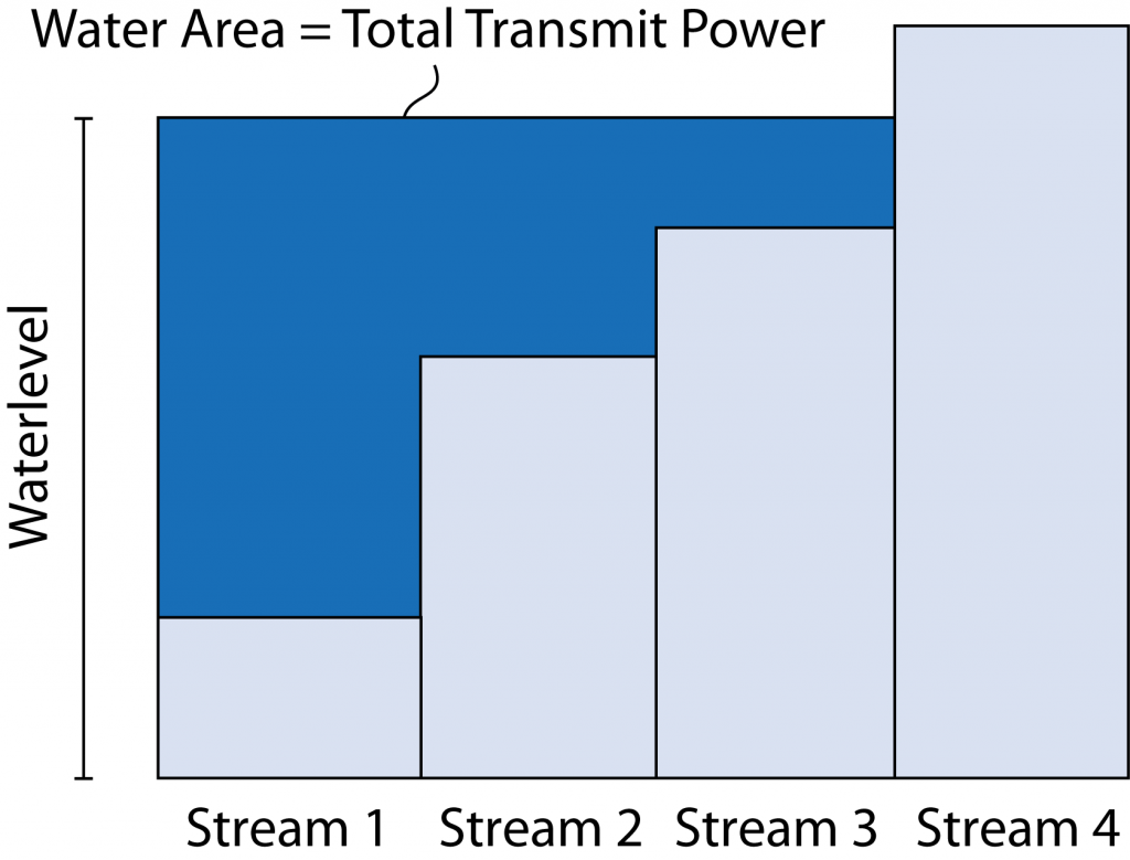
A basic example of this principle arises when communicating over a single-user MIMO channel. To maximize the achievable rate, you first need to select how many data streams to spatially multiplex and then determine the precoding and power allocation for these data streams. This appears to be a mixed-integer optimization problem, but Telatar showed in his seminal paper that it can be solved by the water-filling algorithm. More precisely, you relax the problem by assuming that the maximum number of data streams are transmitted and then you let the solution to a convex optimization problem determine how many of the data streams that are assigned non-zero power; this is the optimal number of data streams. Despite the relaxation, the global optimum to the original problem is obtained.
There are other, less known examples of the “relax and conquer” method. Some years ago, I came across the paper “Jointly optimal downlink beamforming and base station assignment“, which has received much less attention than it deserves. The UE-BS association problem, considered in this paper, is non-trivial since some BSs might have many more UEs in their vicinity than other BSs. Nevertheless, the paper shows that one can solve the problem by first relaxing it so that all BSs transmit to all the UEs. The author formulates a relaxed optimization problem where the beamforming vectors (including power allocation) are selected to satisfy each UEs’ SINR constraint, while minimizing the total transmit power. This problem is solved by convex optimization and, importantly, the optimal solution is always such that each UE only receives a non-zero signal power from one of the BSs. Hence, the seemingly difficult combinatorial UE-BS association problem is relaxed to a convex optimization problem, which provides the optimal solution to the original problem!
I have reused this idea in several papers. The first example is “Massive MIMO and Small Cells: Improving Energy Efficiency by Optimal Soft-cell Coordination“, which considers a similar setup but with a maximum transmit power per BS. The consequence of including this practical constraint is that it might happen that some UEs are served by multiple BSs at the optimal solution. These BSs send different messages to the UE, which decode them by successive interference cancelation, thus the solution is still practically achievable.
One practical weakness with the two aforementioned papers is that they take small-scale fading realizations into account in the optimization, thus the problem must be solved once per coherence interval, requiring extremely high computational power. More recently, in the paper “Joint Power Allocation and User Association Optimization for Massive MIMO Systems“, we applied the same “relax and conquer” method to Massive MIMO, but targeting lower bounds on the downlink ergodic capacity. Since the capacity bounds are valid as long as the channel statistics are fixed (and the same UEs are active), our optimized BS-UE association can be utilized for a relatively long time period. This makes the proposed algorithm practically relevant, in contrast to the prior works that are more of academic interest.
Another example of the “relax and conquer” method is found in the paper “Joint Pilot Design and Uplink Power Allocation in Multi-Cell Massive MIMO Systems”. We consider the assignment of orthogonal pilot sequences to users, which appears to be a combinatorial problem. Instead of assigning a pilot sequence to each UE and then allocate power, we relax the problem by allowing each user to design its own pilot sequence, which is a linear combination of the original orthogonal sequences. Hence, a pair of UEs might have partially overlapping sequences, instead of either identical or orthogonal sequences (as in the original problem). The relaxed problem even allows for pilot contamination within a cell. The sequences are then optimized to maximize the max-min performance. The resulting problem is non-convex, but the combinatorial structure has been relaxed so that there are only optimization variables from continuous sets. A local optimum to the joint pilot assignment and power control problem is found with polynomial complexity, using standard methods from the optimization literature. The optimization might not lead to a set of orthogonal pilot sequences, but the solution is practically implementable and gives better performance.

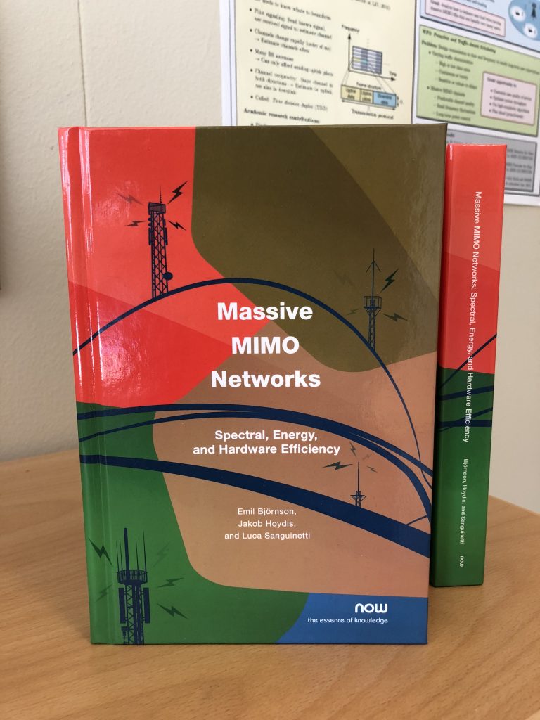 The hardback version of the massive new book Massive MIMO Networks: Spectral, Energy, and Hardware Efficiency (by Björnson, Sanguinetti, Hoydis) is currently available for the special price of $70 (including worldwide shipping). The original price is $99.
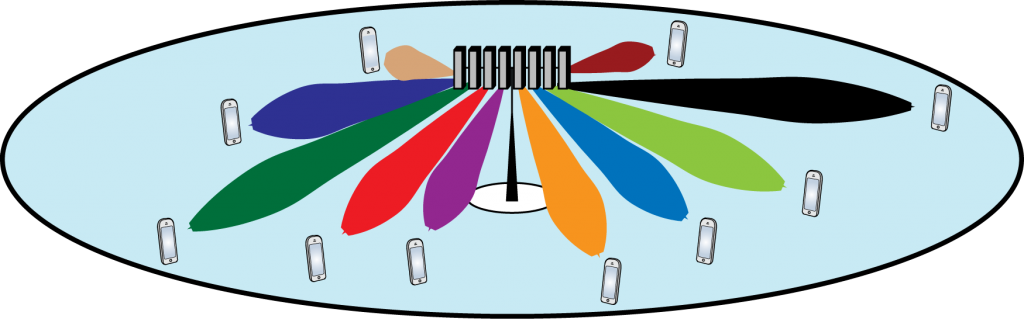

 is the number of base-station antennas,
  is the number of spatially multiplexed users,
 ![$c_{ \textrm{\tiny CSI}} \in [0,1]$](https://ma-mimo.ellintech.se/wp-content/ql-cache/quicklatex.com-638fe579c728859336f107711790c035_l3.png "Rendered by QuickLaTeX.com") is the quality of the channel estimates, and
is the quality of the channel estimates, and  is the number of channel uses per channel coherence block. For simplicity, I have assumed the same pathloss for all the users. The variable
  is the nominal signal-to-noise ratio (SNR) of a user, achieved when
  . Eq. (1) is a rigorous lower bound on the sum capacity, achieved under the assumptions of maximum ratio precoding, i.i.d. Rayleigh fading channels, and equal power allocation. With better processing schemes, one can achieve substantially higher performance.
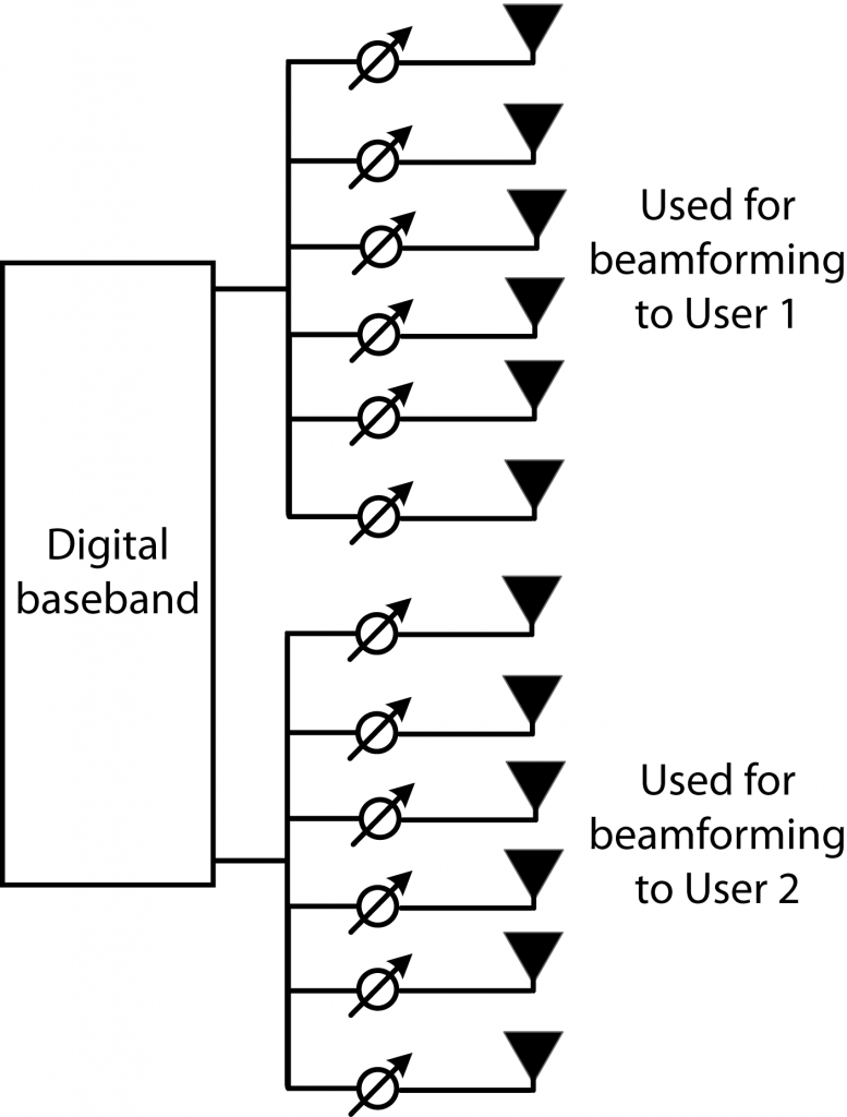
 and, hence, I am a bit concerned that the industry will be disappointed with the gains that they will obtain from such beamforming in 5G.
 stays constant, then the spectral efficiency will grow linearly with the number of users. Note that the same transmit power is divided between the
  and
and  , the spectral efficiency will become 5.6 bit/s/Hz. This is the gain from beamforming. If we also increase the number of users to
  users, we will get 32 bit/s/Hz. This is the gain from spatial multiplexing. Clearly, the largest gains come from spatial multiplexing and adding many antennas is a necessary way to facilitate such multiplexing.
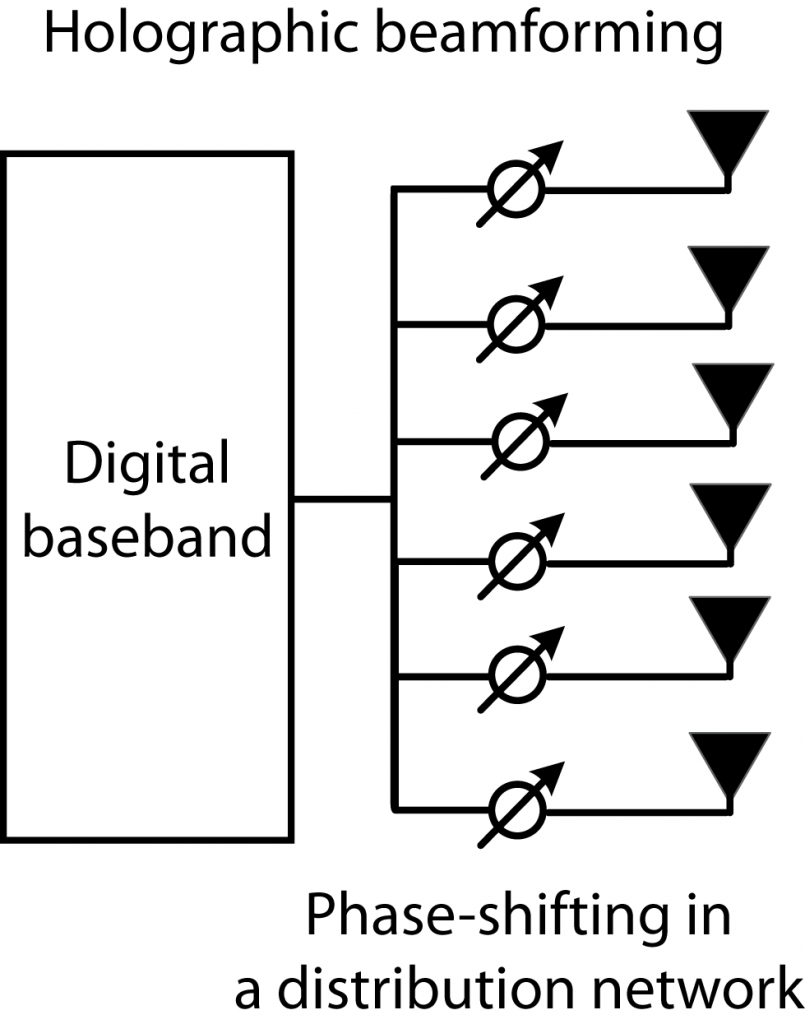 Will the futuristic-sounding holographic beamforming make Massive MIMO obsolete? Not at all, because this is a new implementation architecture, not a new beamforming scheme or spatial multiplexing method. According to the