Yes, my group had its share of rejected papers as well. Here are some that I specially remember:
Massive MIMO: 10 myths and one critical question. The first version was rejected by the IEEE Signal Processing Magazine. The main comment was that nobody would think that the points that we had phrased as myths were true. But in reality, each one of the myths was based on an actual misconception heard in public discussions! The paper was eventually published in the IEEE Communications Magazine instead in 2016, and has been cited more than 180 times.
Massive MIMO with 1-bit ADCs. This paper was rejected by the IEEE Transactions on Wireless Communications. By no means a perfect paper… but the review comments were mostly nonsensical. The editor stated: “The concept as such is straightforward and the conceptual novelty of the manuscript is in that sense limited.” The other authors left my group shortly after the paper was written. I did not predict the hype on 1-bit ADCs for MIMO that would ensue (and this happened despite the fact that yes, the concept as such is straightforward and its conceptual novelty is rather limited!). Hence I didn’t prioritize a rewrite and resubmission. The paper was never published, but we put the rejected manuscript on arXiv in 2014, and it has been cited 80 times.
Finally, a paper that was almost rejected upon its initial submission: Energy and Spectral Efficiency of Very Large Multiuser MIMO Systems, eventually published in the IEEE Transactions on Communications in 2013. The review comments included obvious nonsense, such as “Overall, there is not much difference in theory compared to what was studied in the area of MIMO for the last ten years.” The paper subsequently won the IEEE ComSoc Stephen O. Rice Prize, and has more than 1300 citations.
There are several lessons to learn here. First, that peer review may be the best system we know, but it isn’t perfect: disturbingly, it is often affected by incompetence and bias. Second, notwithstanding the first, that many paper rejections are probably also grounded in genuine misunderstandings: writing well takes a lot of experience, and a lot of hard, dedicated work. Finally, and perhaps most significantly, that persistence is really an essential component of success.
I’ve got an email with this question last week. There is not one but many possible answers to this question, so I figured that I write a blog post about it.
One answer is that beamforming and precoding are two words for exactly the same thing, namely to use an antenna array to transmit one or multiple spatially directive signals.
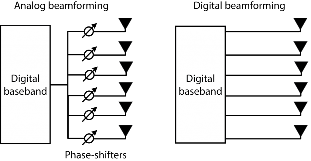
Another answer is that beamforming can be divided into two categories: analog and digital beamforming. In the former category, the same signal is fed to each antenna and then analog phase-shifters are used to steer the signal emitted by the array. This is what a phased array would do. In the latter category, different signals are designed for each antenna in the digital domain. This allows for greater flexibility since one can assign different powers and phases to different antennas and also to different parts of the frequency bands (e.g., subcarriers). This makes digital beamforming particularly desirable for spatial multiplexing, where we want to transmit a superposition of signals, each with a separate directivity. It is also beneficial when having a wide bandwidth because with fixed phases the signal will get a different directivity in different parts of the band. The second answer to the question is that precoding is equivalent to digital beamforming. Some people only mean analog beamforming when they say beamforming, while others use the terminology for both categories.
Analog beamforming uses phase-shifters to send the same signal from multiple antennas but with different phases. Digital beamforming designs different signals for each antennas in the digital baseband. Precoding is sometimes said to be equivalent to digital beamforming.
A third answer is that beamforming refers to a single-user transmission with one data stream, such that the transmitted signal consists of one main-lobe and some undesired side-lobes. In contrast, precoding refers to the superposition of multiple beams for spatial multiplexing of several data streams.
A fourth answer is that beamforming refers to the formation of a beam in a particular angular direction, while precoding refers to any type of transmission from an antenna array. This definition essentially limits the use of beamforming to line-of-sight (LoS) communications, because when transmitting to a non-line-of-sight (NLoS) user, the transmitted signal might not have a clear angular directivity. The emitted signal is instead matched to the multipath propagation so that the multipath components that reach the user add constructively.
A fifth answer is that precoding consists of two parts: choosing the directivity (beamforming) and choosing the transmit power (power allocation).
I used to use the word beamforming in its widest meaning (i.e., the first answer), as can be seen in my first book on the topic. However, I have since noticed that some people have a more narrow or specific interpretation of beamforming. Therefore, I nowadays prefer only talking about precoding. In Massive MIMO, I think that precoding is the right word to use since what I advocate is a fully digital implementation, where the phases and powers can be jointly designed to achieve high capacity through spatial multiplexing of many users, in both NLoS and LOS scenarios.
The “Massive MIMO” name is currently being used for both sub-6 GHz and mmWave applications. This can be very confusing because the multi-antenna technology has rather different characteristics in these two applications.
The sub-6 GHz spectrum is particularly useful to provide network coverage, since the pathloss and channel coherence time are relatively favorable at such frequencies (recall that the coherence time is inversely proportional to the carrier frequency). Massive MIMO at sub-6 GHz spectrum can increase the efficiency of highly loaded cells, by upgrading the technology at existing base stations. In contrast, the huge available bandwidths in mmWave bands can be utilized for high-capacity services, but only over short distances due to the severe pathloss and high noise power (which is proportional to the bandwidth). Massive MIMO in mmWave bands can thus be used to improve the link budget.
Six key differences between sub-6 GHz and mmWave operation are provided below:
Sub-6 GHz
mmWave
Deployment scenario
Macro cells with support for high user mobility
Small cells with low user mobility
Number of simultaneous users per cell
Up to tens of users, due to the large coverage area
One or a few users, due to the small coverage area
Main benefit from having many antennas
Spatial multiplexing of tens of users, since the array gain and ability to separate users spatially lead to great spectral efficiency
Beamforming to a single user, which greatly improves the link budget and thereby extends coverage
Channel characteristics
Rich multipath propagation
Only a few propagation paths
Spectral efficiency and bandwidth
High spectral efficiency due to the spatial multiplexing, but small bandwidth
Low spectral efficiency due to few users, large pathloss, and large noise power, but large bandwidth
Transceiver hardware
Fully digital transceiver implementations are feasible and have been prototyped
Hybrid analog-digital transceiver implementations are needed, at least in the first products
Since Massive MIMO was initially proposed by Tom Marzetta for sub-6 GHz applications, I personally recommend to use the “Massive MIMO” name only for that use case. One can instead say “mmWave Massive MIMO” or just “mmWave” when referring to multi-antenna technologies for mmWave bands.
The received signal power is proportional to the number of antennas in Massive MIMO systems. This property is known as the array gain and it can basically be utilized in two different ways.
One option is to let the signal power become times larger than in a single-antenna reference scenario. The increase in SNR will then lead to higher data rates for the users. The gain can be anything from bit/s/Hz to almost negligible, depending on how interference-limited the system is. Another option is to utilize the array gain to reduce the transmit power, to maintain the same SNR as in the reference scenario. The corresponding power saving can be very helpful to improve the energy efficiency of the system.
In the uplink, with single-antenna user terminals, we can choose between these options. However, in the downlink, we might not have a choice. There are strict regulations on the permitted level of out-of-band radiation in practical systems. Since Massive MIMO uses downlink precoding, the transmitted signals from the base station have a stronger directivity than in the single-antenna reference scenario. The signal components that leak into the bands adjacent to the intended frequency band will then also be more directive.
For example, consider a line-of-sight scenario where the precoding creates an angular beam towards the intended user (as illustrated in the figure below). The out-of-band radiation will then get a similar angular directivity and lead to larger interference to systems operating in adjacent bands, if their receivers are close to the user (as the victim in the figure below). To counteract this effect, our only choice might be to reduce the downlink transmit power to keep the worst-case out-of-band radiation constant.
Another alternative is that the regulations are made more flexible with respect to precoded transmissions. The probability that a receiver in an adjacent band is hit by an interfering out-of-band beam, such that the interference becomes times larger than in the reference scenario, reduces with an increasing number of antennas since the beams are narrower. Hence, if one can allow for beamformed out-of-band interference if it occurs with sufficiently low probability, the array gain in Massive MIMO can still be utilized to increase the SNRs. A third option will then be to (partially) reduce the transmit power to also allow for relaxed linearity requirements of the hardware.
Many researchers have analyzed pilot contamination over the six years that have passed since Marzetta uncovered its importance in Massive MIMO systems. We now have a quite good understanding of how to mitigate pilot contamination. There is a plethora of different approaches, whereof many have complementary benefits. If pilot contamination is not mitigated, it will both reduce the array gain and create coherent interference. Some approaches mitigate the pilot interference in the channel estimation phase, while some approaches combat the coherent interference caused by pilot contamination. In this post, I will try to categorize the approaches and point to some key references.
Interference-rejecting precoding and combining
Pilot contamination makes the estimate of a desired channel correlated with the channel from pilot-sharing users in other cells. When these channel estimates are used for receive combining or transmit precoding, coherent interference typically arise. This is particularly the case if maximum ratio processing is used, because it ignores the interference. If multi-cell MMSE processing is used instead, the coherent interference is rejected in the spatial domain. In particular, recent work from Björnson et al. (see also this related paper) have shown that there is no asymptotic rate limit when using this approach, if there is just a tiny amount of spatial correlation in the channels.
Data-aided channel estimation
Another approach is to “decontaminate” the channel estimates from pilot contamination, by using the pilot sequence and the uplink data for joint channel estimation. This have the potential of both improving the estimation quality (leading to a stronger desired signal) and reducing the coherent interference. Ideally, if the data is known, data-aided channel estimation increase the length of the pilot sequences to the length of the uplink transmission block. Since the data is unknown to the receiver, semi-blind estimation techniques are needed to obtain the channel estimates. Ngo et al. and Müller et al. did early works on pilot decontamination for Massive MIMO. Recent work has proved that one can fully decontaminate the estimates, as the length of the uplink block grows large, but it remains to find the most efficient semi-blind decontamination approach for practical block lengths.
Pilot assignment and dimensioning
Which subset of users that share a pilot sequence makes a large difference, since users with large pathloss differences and different spatial channel correlation cause less contamination to each other. Recall that higher estimation quality both increases the gain of the desired signal and reduces the coherent interference. Increasing the number of orthogonal pilot sequences is a straightforward way to decrease the contamination, since each pilot can be assigned to fewer users in the network. The price to pay is a larger pilot overhead, but it seems that a reuse factor of 3 or 4 is often suitable from a sum rate perspective in cellular networks. The joint spatial division and multiplexing (JSDM) provides a basic methodology to take spatial correlation into account in the pilot reuse patterns.
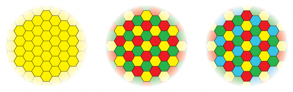
A cellular network with different pilot reuse factors: Reuse 1 (left), Reuse 3 (middle), Reuse 4 (right). The cells with the same color uses the same subset of pilots.
Alternatively, pilot sequences can be superimposed on the data sequences, which gives as many orthogonal pilot sequences as the length of the uplink block and thereby reduces the pilot contamination. This approach also removes the pilot overhead, but it comes at the cost of causing interference between pilot and data transmissions. It is therefore important to assign the right fraction of power to pilots and data. A hybrid pilot solution, where some users have superimposed pilots and some have conventional pilots, may bring the best of both worlds.
If two cells use the same subset of pilots, the exact pilot-user assignment can make a large difference. Cell-center users are generally less sensitive to pilot contamination than cell-edge users, but finding the best assignment is a hard combinatorial problem. There are heuristic algorithms that can be used and also an optimization framework that can be used to evaluate such algorithms.
Multi-cell cooperation
A combination of network MIMO and macro diversity can be utilized to turn the coherent interference into desired signals. This approach is called pilot contamination precoding by Ashikhmin et al. and can be applied in both uplink and downlink. In the uplink, the base stations receive different linear combinations of the user signals. After maximum ratio combining, the coefficients in the linear combinations approach deterministic numbers as the number of antennas grow large. These numbers are only non-zero for the pilot-sharing users. Since the macro diversity naturally creates different linear combinations, the base stations can jointly solve a linear system of equations to obtain the transmitted signals. In the downlink, all signals are sent from all base stations and are precoded in such a way that the coherent interference sent from different base stations cancel out. While this is a beautiful approach for mitigating the coherent interference, it relies heavily on channel hardening, favorable propagation, and i.i.d. Rayleigh fading. It remains to be shown if the approach can provide performance gains under more practical conditions.
Since its inception, Massive MIMO has been strongly connected with asymptotic analysis. Marzetta’s seminal paper featured an unlimited number of base station antennas. Many of the succeeding papers considered a finite number of antennas, , and then analyzed the performance in the limit where . Massive MIMO is so tightly connected with asymptotic analysis that reviewers question whether a paper is actually about Massive MIMO if it does not contain an asymptotic part – this has happened to me repeatedly.
Have you reflected over what the purpose of asymptotic analysis is? The goal is not that we should design and deploy wireless networks with a nearly infinite number of antennas. Firstly, it is physically impossible to do that in a finite-sized world, irrespective of whether you let the array aperture grow or pack the antennas more densely. Secondly, the conventional channel models break down, since you will eventually receive more power than you transmitted. Thirdly, the technology will neither be cost nor energy efficient, since the cost/energy grows linearly with , while the delivered system performance either approaches a finite limit or grows logarithmically with .
It is important not to overemphasize the implications of asymptotic results. Consider the popular power-scaling law which says that one can use the array gain of Massive MIMO to reduce the transmit power as and still approach a non-zero asymptotic rate limit. This type of scaling law has been derived for many different scenarios in different papers. The practical implication is that you can reduce the transmit power as you add more antennas, but the asymptotic scaling law does not prescribe how much you should reduce the power when going from, say, 40 to 400 antennas. It all depends on which rates you want to deliver to your users.
The figure below shows the transmit power in a scenario where we start with 1 W for a single-antenna transmitter and then follow the asymptotic power-scaling law as the number of antennas increases. With antennas, the transmit power per antenna is just 1 mW, which is unnecessarily low given the fact that the circuits in the corresponding transceiver chain will consume much more power. By using higher transmit power than 1 mW per antenna, we can deliver higher rates to the users, while barely effecting the total power of the base station.
Reducing the transmit power per antenna to 1 mW, or smaller, makes little practical sense, since the transceiver chain will consume much more power irrespective of the transmit power.
Similarly, there is a hardware-scaling law which says that one can increase the error vector magnitude (EVM) proportionally to and approach a non-zero asymptotic rate limit. The practical implication is that Massive MIMO systems can use simpler hardware components (that cause more distortion) than conventional systems, since there is a lower sensitivity to distortion. This is the foundation on which the recent works on low-bit ADC resolutions builds (see this paper and references therein).
Even the importance of the coherent interference, caused by pilot contamination, is easily overemphasized if one only considers the asymptotic behavior. For example, the finite rate limit that appears when communicating over i.i.d. Rayleigh fading channels with maximum ratio or zero-forcing processing is only approached in practice if one has around one million antennas.
In my opinion, the purpose of asymptotic analysis is not to understand the asymptotic behaviors themselves, but what the asymptotics can tell us about the performance at practical number of antennas. Here are some usages that I think are particularly sound:
Determine what is the asymptotically optimal transmission scheme and then evaluate how it performs in a practical system.
Derive large-scale approximations of the rates that are reasonable tight also at practical number of antennas. One can use these approximations to determine which factors that have a dominant impact on the rate or to get a tractable way to optimize system performance (e.g., by transmit power allocation).
Determine how far from the asymptotically achievable performance a practical system is.
Simplify the signal processing by utilizing properties such as channel hardening and favorable propagation. These phenomena can be observed already at 100 antennas, although you will never get a fully deterministic channel or zero inter-user interference in practice.
Some form of Massive MIMO will appear in 5G, but to get a well-designed system we need to focus more on demonstrating and optimizing the performance in practical scenarios (e.g., the key 5G use cases) and less on pure asymptotic analysis.
The channel between a single-antenna user and an -antenna base station can be represented by an -dimensional channel vector. The canonical channel model in the Massive MIMO literature is independent and identically distributed (i.i.d.) Rayleigh fading, in which the vector is a circularly symmetric complex Gaussian random variable with a scaled identity matrix as correlation/covariance matrix: , where is the variance.
With i.i.d. Rayleigh fading, the channel gain has an Erlang-distribution (this is a scaled distribution) and the channel direction is uniformly distributed over the unit sphere in . The channel gain and the channel direction are also independent random variables, which is why this is a spatially uncorrelated channel model.
One of the key benefits of i.i.d. Rayleigh fading is that one can compute closed-form rate expressions, at least when using maximum ratio or zero-forcing processing; see Fundamentals of Massive MIMO for details. These expressions have an intuitive interpretation, but should be treated with care because practical channels are not spatially uncorrelated. Firstly, due to the propagation environment, the channel vector is more probable to point in some directions than in others. Secondly, the antennas have spatially dependent antenna patterns. Both factors contribute to the fact that spatial channel correlation always appears in practice.
One of the basic properties of spatial channel correlation is that the base station array receives different average signal power from different spatial directions. This is illustrated in Figure 1 below for a uniform linear array with 100 antennas, where the angle of arrival is measured from the boresight of the array.
Figure 1: The average signal power received at a Massive MIMO base station from different angular directions, as seen from the array. Spatially correlated fading implies that this average power is angle-dependent, while i.i.d. fading gives the same power in all directions.
As seen from Figure 1, with i.i.d. Rayleigh fading the average received power is equally large from all directions, while with spatially correlated fading it varies depending on in which direction the base station applies its receive beamforming. Note that this is a numerical example that was generated by letting the signal come from four scattering clusters located in different angular directions. Channel measurements from Lund University (see Figure 4 in this paper) show how the spatial correlation behaves in practical scenarios.
Correlated Rayleigh fading is a tractable way to model a spatially correlation channel vector: , where the covariance matrix is also the correlation matrix. It is only when is a scaled identity matrix that we have spatially uncorrelated fading. The eigenvalue distribution determines how strongly spatially correlated the channel is. If all eigenvalues are identical, then is a scaled identity matrix and there is no spatial correlation. If there are a few strong eigenvalues that contain most of the power, then there is very strong spatial correlation and the channel vector is very likely to be (approximately) spanned by the corresponding eigenvectors. This is illustrated in Figure 2 below, for the same scenario as in the previous figure. In the considered correlated fading case, there are 20 eigenvalues that are larger than in the i.i.d. fading case. These eigenvalues contain 94% of the power, while the next 20 eigenvalues contain 5% and the smallest 60 eigenvalues only contain 1%. Hence, most of the power is concentrated to a subspace of dimension . The fraction of strong eigenvalues is related to the fraction of the angular interval from which strong signals are received. This relation can be made explicit in special cases.
Figure 2: Spatial channel correlation results in eigenvalue variations, while all eigenvalues are the same under i.i.d fading. The larger the variations, the stronger the correlation is.
One example of spatially correlated fading is when the correlation matrix has equal diagonal elements and non-zero off-diagonal elements, which describe the correlation between the channel coefficients of different antennas. This is a reasonable model when deploying a compact base station array in tower. Another example is a diagonal correlation matrix with different diagonal elements. This is a reasonable model when deploying distributed antennas, as in the case of cell-free Massive MIMO.
Finally, a more general channel model is correlated Rician fading: , where the mean value represents the deterministic line-of-sight channel and the covariance matrix determines the properties of the fading. The correlation matrix can still be used to determine the spatial correlation of the received signal power. However, from a system performance perspective, the fraction between the power of the line-of-sight path and the scattered paths can have a large impact on the performance as well. A nearly deterministic channel with a large -factor provide more reliable communication, in particular since under correlated fading it is only the large eigenvalues of that contributes to the channel hardening (which otherwise provides reliability in Massive MIMO).

 in Massive MIMO systems. This property is known as the array gain and it can basically be utilized in two different ways.
 bit/s/Hz to almost negligible, depending on how interference-limited the system is. Another option is to utilize the array gain to reduce the transmit power, to maintain the same SNR as in the reference scenario. The corresponding power saving can be very helpful to improve the energy efficiency of the system.
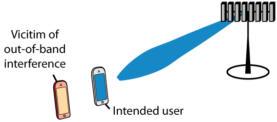
 . Massive MIMO is so tightly connected with asymptotic analysis that reviewers question whether a paper is actually about Massive MIMO if it does not contain an asymptotic part – this has happened to me repeatedly.
 and still approach a non-zero asymptotic rate limit. This type of scaling law has been derived for many different scenarios in different papers. The practical implication is that you can reduce the transmit power as you add more antennas, but the asymptotic scaling law does not prescribe how much you should reduce the power when going from, say, 40 to 400 antennas. It all depends on which rates you want to deliver to your users.
 antennas, the transmit power per antenna is just 1 mW, which is unnecessarily low given the fact that the circuits in the corresponding transceiver chain will consume much more power. By using higher transmit power than 1 mW per antenna, we can deliver higher rates to the users, while barely effecting the total power of the base station.
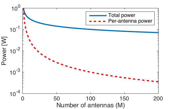
 and approach a non-zero asymptotic rate limit. The practical implication is that Massive MIMO systems can use simpler hardware components (that cause more distortion) than conventional systems, since there is a lower sensitivity to distortion. This is the foundation on which the recent works on low-bit ADC resolutions builds (
 , where
  is the variance.
 has an
  -distribution (this is a scaled
  distribution) and the channel direction
  is uniformly distributed over the unit sphere in
  . The channel gain and the channel direction are also independent random variables, which is why this is a spatially uncorrelated channel model.
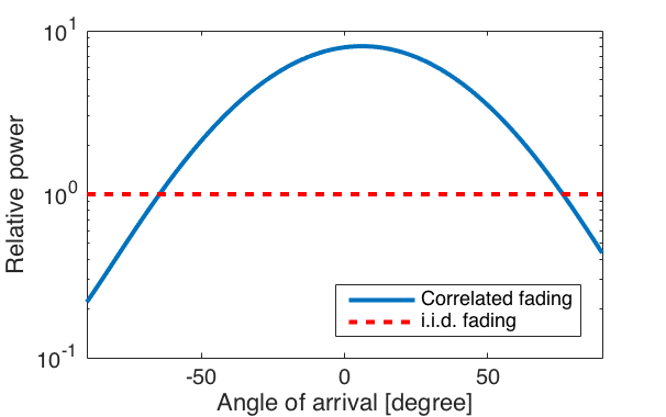
 , where the covariance matrix
  is also the correlation matrix. It is only when
  . The fraction of strong eigenvalues is related to the fraction of the angular interval from which strong signals are received.
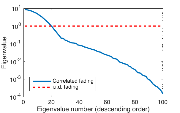
 , where the mean value
  represents the deterministic line-of-sight channel and the covariance matrix
  can still be used to determine the spatial correlation of the received signal power. However, from a system performance perspective, the fraction
  between the power of the line-of-sight path and the scattered paths can have a large impact on the performance as well. A nearly deterministic channel with a large
  -factor provide more reliable communication, in particular since under correlated fading it is only the large eigenvalues of