Category Archives: Commentary

Pilot Contamination is Not Captured by the MSE

Pilot contamination used to be seen as the key issue with the Massive MIMO technology, but thanks to a large number of scientific papers we now know fairly well how to deal with it. I outlined the main approaches to mitigate pilot contamination in a previous blog post and since then the paper Massive MIMO has unlimited capacity has also been picked up by science news channels.

When reading papers on pilot (de)contamination written by many different authors, I’ve noticed one recurrent issue: the mean-squared error (MSE) is used to measure the level of pilot contamination. A few papers only plot the MSE, while most papers contain multiple MSE plots and then one or two plots with bit-error-rates or achievable rates. As I will explain below, the MSE is a rather poor measure of pilot contamination since it cannot distinguish between noise and pilot contamination.

A simple example

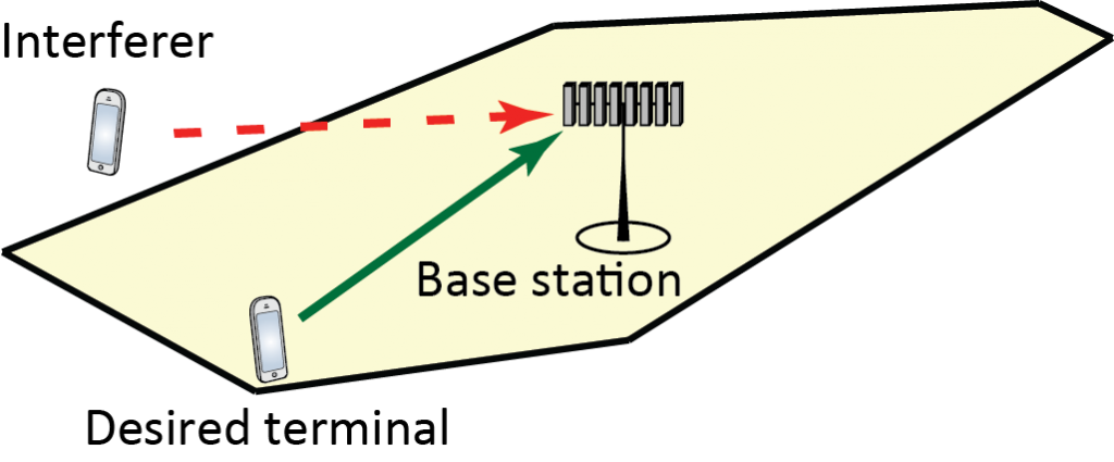
Suppose the desired uplink signal is received with power p and is disturbed by noise with power (1-a) and interference from another user with power a. By varying the variable a between 0 and 1 in this simple example, we can study how the performance changes when moving power from the noise to the interference, and vice versa.

By following the standard approach for channel estimation based on uplink pilots (see Fundamentals of Massive MIMO), the MSE for i.i.d. Rayleigh fading channels is

    $$\textrm{MSE} = \frac{p}{p+(1-a)+a} = \frac{p}{p+1}, $$

which is independent of a and, hence, does not care about whether the disturbance comes from noise or interference. This is rather intuitive since both the noise and interference are additive i.i.d. Gaussian random variables in this example. The important difference appears in the data transmission phase, where the noise takes a new independent realization and the interference is strongly correlated with the interference in the pilot phase, because it is the product of a new scalar signal and the same channel vector.

To demonstrate the important difference, suppose maximum ratio combining is used to detect the uplink data. The effective uplink signal-to-interference-and-noise-ratio (SINR) is

    $$\textrm{SINR} = \frac{p(1-\textrm{MSE}) M}{p+1+a M \cdot \textrm{MSE}}$$

where M is the number of antennas. For any given MSE value, it now matters how it was generated, because the SINR is a decreasing function of a. The term a M  \cdot \textrm{MSE} is due to pilot contamination (it is often called coherent interference) and is proportional to the interference power $a$. When the number of antennas is large, it is far better to have more noise during the pilot transmission than more interference!

Implications

Since the MSE cannot separate noise from interference, we should not try to measure the effectiveness of a “pilot decontamination” algorithm by considering the MSE. An algorithm that achieves a low MSE can potentially be mitigating the noise, leaving the interference unaffected. If that is the case, the pilot contamination term $a M  \cdot \textrm{MSE}$ will remain. The MSE has been used far too often when evaluating pilot decontamination algorithms, and a few papers (I found three while writing this post) did only consider the MSE, which opens the door for questioning their conclusions.

The right methodology is to compute the SINR (or some other performance indicator in the data phase) with the proposed pilot decontamination algorithm and with competing algorithms. In that case, we can be sure that the full impact of the pilot contamination is taken into account.

Massive MIMO for Maritime Communications

The Norwegian startup company Super Radio has during the past year made several channel measurement campaigns for Massive MIMO for land-to-sea communications, within a project called MAMIME (LTE, WIFI and 5G Massive MIMO Communications in Maritime Propagation Environments). There are several other companies and universities involved in the project.

The maritime propagation environment is clearly different from the urban and suburban propagation environments that are normally modeled in wireless communications. For example, the ground plane consists of water, and the sea waves are likely to reflect the radio waves in a different way than the hard surface on land. Except for islands, there won’t be many other objects that can create multipath propagation in the sea. Hence, a strong line-of-sight path is key in these use cases.

The MAMIME project is using a 128-antenna horizontal array, which is claimed to be the largest in the world. Such an array can provide narrow horizontal beams, but no elevation beamforming – which is probably not needed since the receivers will all be at the sea level. The array consists of 4 subarrays which each has a dimension of 1070 x 630 mm. Frequencies relevant for LTE and WiFi have been considered so far. The goal of the project is to provide “extremely high throughputs, stability and long coverage” for maritime communications. I suppose that range extension and spatial multiplexing of multiple ships is what this type of Massive MIMO system can achieve, as compared to a conventional system.

A first video about the project was published in December 2017:

Now a second video has been released, see below. Both videos have been recorded outside Trondheim, but Kan Yang at Super Radio told me that further measurements outside Oslo will soon be conducted, with focus on LTE Massive MIMO.

A Look at an LTE-TDD Massive MIMO Product

I wrote earlier about the Ericsson AIR 6468 that was deployed in Russian in preparation for the 2018 World Cup in football. If you are curious to know more about this Massive MIMO product, among the first of its kind, you can read the public documents that were submitted to FCC for approval. For example, if you click on the link above and then select “Conf Exhibit 9 Internal photos” you will see how the product looks at the inside.

I will now summarize some of the key properties of this LTE TDD product. AIR stands for Antenna Integrated Radio, and Ericsson AIR 6468 is a unit with 64 antennas connected to 64 transmitter/receiver branches. This allows for fully digital beamforming, but the baseband processing is taking place in a separate unit that is connected to AIR 6468 with an optical cable. Hence, the processing unit can be updated to support future LTE releases and more advanced signal processing.

There are different versions of AIR 6468 that are targeting different LTE bands, for example, 2496-2690 MHz and 3400–3600 MHz. These units weight 60.4 kg and are 988 x 520 x 187 mm, which clearly demonstrates that Massive MIMO does not require physically large arrays; the height is typical for an LTE antenna, while the width is slightly larger. This can be seen in the image below, where the AIR 6468 is in the middle.


The array can be mounted on a wall or a pole, and tilted in various ways. As far as I understand, the 64 antennas consist of 32 dual-polarized antennas, which are arranged on a rectangular grid with 4 antennas in the vertical dimension and 8 antennas in the horizontal dimension. The reason that the array is still physically larger in the vertical dimension is the larger vertical antenna spacing, which is the common practice to achieve a narrower vertical beamwidth since most users are concentrated around the same elevation angles in practical deployments (see Section 7.3-7.4 in Massive MIMO Networks for a more detailed explanation).

QPSK, 16-QAM, 64-QAM, and 256-QAM are the supported modulation types. AIR 6468 can perform carrier aggregation of up to three carriers of 15 or 20 MHz each. The maximum radiated transmit power is 1.875 W per antenna, which corresponds to 120 W in total for the array. I suppose this means 40 W in total in each 15-20 MHz carrier (and 0.625 W per antenna), but it is of course the spectrum licenses that determine the actual numbers.

64 or 128 Antennas?

After some successful trials, the first deployments of TDD-LTE with Massive MIMO functionality were unveiled earlier this year. For example, the telecom operator Sprint turned on Massive MIMO base stations in Chicago, Dallas, and Los Angeles last April.

If you read the press release from Sprint, it is easy to get confused regarding the number of antennas being used:

Sprint will deploy 64T64R (64 transmit, 64 receive) Massive MIMO radios using 128 antennas working with technology leaders Ericsson, Nokia, and Samsung Electronics.

From reading this quote, I get the impression that the Massive MIMO arrays contain 128 antennas, whereof 64 are used for the transmission and another 64 for the reception. That would be a poor system design, since channel reciprocity can only be exploited in TDD if the same antennas are used for both transmission and reception!

Fortunately, this is not what Sprint and other operators have actually deployed. According to my sources, the arrays contain 64 dual-polarized elements, so there are indeed 128 radiating elements. However, as I explained in a previous blog post, an antenna consists of a collection of radiating elements that are connected to the same RF chain. The number of antennas is equal to the number of RF chains, which is 64 in this case. The reason that Sprint points out that there are 64 transmit antennas and 64 receive antennas is because different RF chains are used for transmission and reception. The system switches between them according to the TDD protocol. In principle, one could design an array that has a different number of RF chains in the uplink than in the downlink, but that is not the case here.

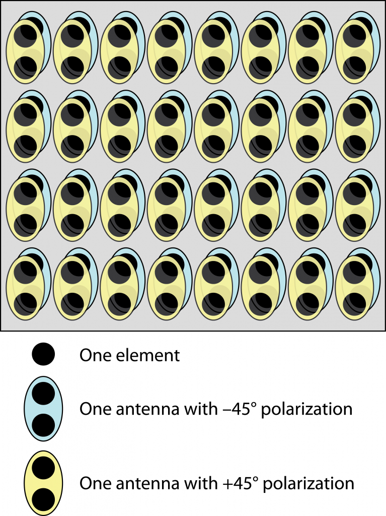
So how are the 128 elements mapped to 64 antennas (RF chains)? This is done by taking pairs of vertically adjacent elements, which have the same polarization, and connecting them to the same RF chain.  This is illustrated in the figure to the right (see this blog post for pictures of how the actual arrays look like). As compared to having 128 RF chains (and antennas), this design choice results in lower flexibility in elevation beamforming, but the losses in data rates and multiplexing capability are supposed to be small since there are much larger variations in azimuth angles between the users in a cellular network than in the elevation angles. (This is explained in detail in Section 7.3-7.4 of my book). The advantage is that the implementation is more compact and less expensive when having 64 instead of 128 antennas.

Massive MIMO at the World Cup

Massive MIMO supports an order of magnitude higher spectral efficiency than legacy LTE networks. The largest gains come from spatial multiplexing of many users per cell, thus these gains can only be harvested when there are many users requesting data at every given millisecond, which requires larger traffic loads than you might think since many seemingly continuous user applications only send data sporadically.

For this reason, I used to say that outdoor musical festivals, where a crowd of 100,000 people gather to see their favorite bands, would be a first deployment scenario for Massive MIMO. This is fairly similar to what now has happened: The Russian telecom operator MTS has deployed more than 40 state-of-the-art LTE sites with Massive MIMO functionality in seven cities where the 2018 FIFA World Cup in football is currently taking place. The base stations are deployed to cover the stadiums, fan zones, airports, train stations, and major parks/squares; in other words, the places where huge crowds of football fans are expected.

In the press release, Andrei Ushatsky, Vice President of MTS, says:

Ericsson AIR 6468 base station array with 64 antennas, which is deployed in Russia

“This launch is one of Europe’s largest Massive MIMO deployments, covering seven Russian cities, and is a major contribution by MTS in the preparation of the country’s infrastructure for the global sporting event of the year. Our Massive MIMO technology, using Ericsson equipment, significantly increases network capacity, allowing tens of thousands of fans together in one place to enjoy high-speed mobile internet without any loss in speed or quality.”

While this is one of the first major deployments of Massive MIMO, more will certainly follow in the coming years. More research into the development and implementation of advanced signal processing and resource management schemes will also be needed for many years to come – this is just the beginning.

Disadvantages with TDD

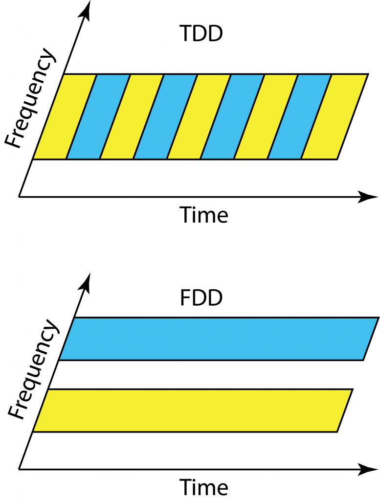
LTE was designed to work equally well in time-division duplex (TDD) and frequency division duplex (FDD) mode, so that operators could choose their mode of operation depending on their spectrum licenses. In contrast, Massive MIMO clearly works at its best in TDD, since the pilot overhead is prohibitive in FDD (even if there are some potential solutions that partially overcome this issue).

Clearly, we will see a larger focus on TDD in future networks, but there are some traditional disadvantages with TDD that we need to bear in mind when designing these networks. I describe the three main ones below.

Link budget

Even if we allocate the same amount of time-frequency resources to uplink and downlink in TDD and FDD operation, there is an important difference. We transmit over half the bandwidth all the time in FDD, while we transmit over the whole bandwidth half of the time in TDD.  Since the power amplifier is only active half of the time, if the peak power is the same, the average radiated power is effectively cut in half. This means that the SNR is 3 dB lower in TDD than in FDD, when transmitting at maximum peak power.

Massive MIMO systems are generally interference-limited and uses power control to assign a reduced transmit power to most users, thus the impact of the 3 dB SNR loss at maximum peak power is immaterial in many cases. However, there will always be some unfortunate low-SNR users (e.g., at the cell edge) that would like to communicate at maximum peak power in both uplink and downlink, and therefore suffer from the 3 dB SNR loss. If these users are still able to connect to the base station, the beamforming gain provided by Massive MIMO will probably more than compensate for the loss in link budget as compared single-antenna systems. One can discuss if it should be the peak power or average radiated power that is constrained in practice.

Guard period

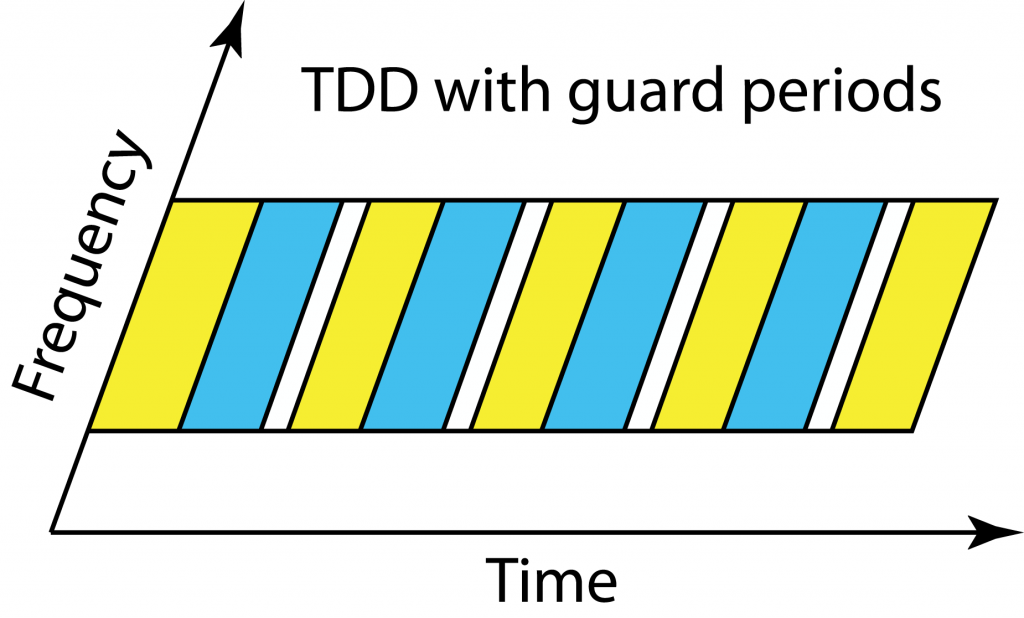
Everyone in the cell should operate in uplink and downlink mode at the same time in TDD. Since the users are at different distances from the base station and have different delay spreads, they will receive the end of the downlink transmission block at different time instances. If a cell center user starts to transmit in the uplink immediately after receiving the full downlink block, then users at the cell edge will receive a combination of the delayed downlink transmission and the cell center users’ uplink transmissions. To avoid such uplink-downlink interference, there is a guard period in TDD so that all users wait with uplink transmission until the outmost users are done with the downlink.

In fact, the base station gives every user a timing bias to make sure that when the uplink commences, the users’ uplink signals are received in a time-synchronized fashion at the base station. Therefore, the outmost users will start transmitting in the uplink before the cell center users. Thanks to this feature, the largest guard period is needed when switching from downlink to uplink, while the uplink to downlink switching period can be short. This is positive for Massive MIMO operation since we want to use uplink CSI in the next downlink block, but not the other way around.

The guard period in TDD must become larger when the cell size increases, meaning that a larger fraction of the transmission resources disappears. Since no guard periods are needed in FDD, the largest benefits of TDD will be seen in urban scenarios where the macro cells have a radius of a few hundred meters and the delay spread is short.

Inter-cell synchronization

We want to avoid interference between uplink and downlink within a cell and the same thing applies for the inter-cell interference. The base stations in different cells should be fairly time-synchronized so that the uplink and downlink take place at the same time; otherwise, it might happen that a cell-edge user receives a downlink signal from its own base station and is interfered by the uplink transmission from a neighboring user that connects to another base station.

This can also be an issue between telecom operators that use neighboring frequency bands. There are strict regulations on the permitted out-of-band radiation, but the out-of-band interference can anyway be larger than the desired inband signal if the interferer is very close to the receiving inband user. Hence, it is preferred that the telecom operators are also synchronizing their switching between uplink and downlink.

Summary

Massive MIMO will bring great gains in spectral efficiency in future cellular networks, but we should not forget about the traditional disadvantages of TDD operation: 3 dB loss in SNR at peak power transmission, larger guard periods in larger cells, and time synchronization between neighboring base stations.

Are 1-bit ADCs Meaningful?

Contemporary base stations are equipped with analog-to-digital converters (ADCs) that take samples described by 12-16 bits. Since the communication bandwidth is up to 100 MHz in LTE Advanced, a sampling rate of a 500 Msample/s is quite sufficient for the ADC. The power consumption of such an ADC is at the order of 1 W. Hence, in a Massive MIMO base station with 100 antennas, the ADCs would consume around 100 W!

ADC SymbolFortunately, the 1600 bit/sample that are effectively produced by 100 16-bit ADCs are much more than what is needed to communicate at practical SINRs. For this reason, there is plenty of research on Massive MIMO base stations equipped with lower-resolution ADCs. The use of 1-bit ADCs has received particular attention. Some good paper references are provided in a previous blog post: Are 1-bit ADCs sufficient? While many early works considered narrowband channels, recent papers (e.g., Quantized massive MU-MIMO-OFDM uplink) have demonstrated that 1-bit ADCs can also be used in practical frequency-selective wideband channels. I’m impressed by the analytical depth of these papers, but I don’t think it is practically meaningful to use 1-bit ADCs.

Do we really need 1-bit ADCs?

I think the answer is no in most situations. The reason is that ADCs with a resolution of around 6 bits strike a much better balance between communication performance and power consumption. The state-of-the-art 6-bit ADCs are already very energy-efficient. For example, the paper “A 5.5mW 6b 5GS/S 4×-lnterleaved 3b/cycle SAR ADC in 65nm CMOS” from ISSCC 2015 describes a 6-bit ADC that consumes 5.5 mW and has a huge sampling rate of 5 Gsample/s, which is sufficient even for extreme mmWave applications with 1 GHz of bandwidth. In a base station equipped with 100 of these 6-bit ADCs, less than 1 W is consumed by the ADCs. That will likely be a negligible factor in the total power consumption of any base station, so what is the point in using a lower resolution than that?

The use of 1-bit ADCs comes with a substantial loss in communication rate. In contrast, there is a consensus that Massive MIMO with 3-5 bits per ADC performs very close to the unquantized case (see Paper 1Paper 2, Paper 3, Paper 4Paper 5). The same applies for 6-bit ADCs, which provide an additional margin that protects against strong interference. Note that there is nothing magical with 6-bit ADCs; maybe 5-bit or 7-bit ADCs will be even better, but I don’t think it is meaningful to use 1-bit ADCs.

Will 1-bit ADCs ever become useful?

To select a 1-bit ADC, instead of an ADC with higher resolution, the energy consumption of the receiving device must be extremely constrained. I don’t think that will ever be the case in base stations, because the power amplifiers are dominating their energy consumption. However, the case might be different for internet-of-things devices that are supposed to run for ten years on the same battery. To make 1-bit ADCs meaningful, we need to greatly simplify all the other hardware components as well. One potential approach is to make a dedicated spatial-temporal waveform design, as described in this paper.