All posts by Erik G. Larsson

Massive MIMO at 60 GHz vs. 2 GHz: How Many More Antennas?

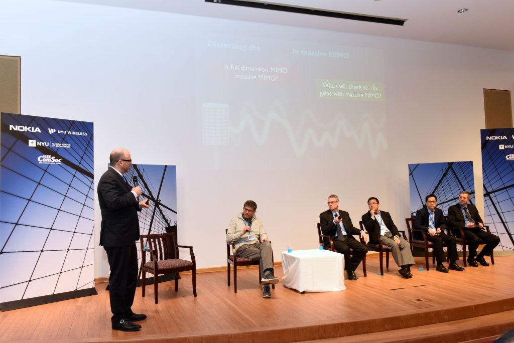
The Brooklyn summit last week was a great event. I gave a talk (here are the slides) comparing MIMO at “PCS” (2 GHz) and mmWave (60 GHz) in line-of-sight. There are two punchlines: first, scientifically, while a link budget calculation might predict that 128.000 mmWave antennas are needed to match up the performance of 128-antenna PCS MIMO, there is a countervailing effect in that increasing the number of antennas improves channel orthogonality so that only 10.000 antennas are required. Second, practically, although 10.000 is a lot less than 128.000, it is still a very large number! Here is a writeup with some more detail on the comparison.

I also touched the (for sub-5 GHz bands somewhat controversial) topic of hybrid beamforming, and whether that would reduce the required amount of hardware.

A question from the audience was whether the use of antennas with larger physical aperture (i.e., intrinsic directivity) would change the conclusions. The answer is no: the use of directional antennas is more or less equivalent to sectorization. The problem is that to exploit the intrinsic gain, the antennas must a priori point “in the right direction”. Hence, in the array, only a subset of the antennas will be useful when serving a particular terminal. This impacts both the channel gain (reduced effective aperture) and orthogonality (see, e.g, Figure 7.5 in this book).

There was also a stimulating panel discussion afterwards. One question discussed in the panel concerned the necessity, or desirability, of using multiple terminal antennas at mmWave. Looking only at the link budget, base station antennas could be traded against terminal antennas – however, that argument neglects the inevitably lost orthogonality, and furthermore it is not obvious how beam-finding/tracking algorithms will perform (millisecond coherence time at pedestrian speeds!). Also, obviously, the comparison I presented is extremely simplistic – to begin with, the line-of-sight scenario is extremely favorable for mmWaves (blocking problems), but also, I entirely neglected polarization losses. Solely any attempts to compensate for these problems are likely to require multiple terminal antennas.

Other topics touched in the panel were the viability of Massive MIMO implementations. Perhaps the most important comment in this context made was by Ian Wong of National Instruments: “In the past year, we’ve actually shown that [massive MIMO] works in reality … To me, the biggest development is that the skeptics are being quiet.” (Read more about that here.)

Real-Time Massive MIMO DSP at 50 milliWatt

Colleagues at Lund University presented last month a working circuit that performs, in real time, zero-forcing decoding and precoding of 8 simultaneous terminals with 128 base station antennas, over a 20 MHz bandwidth at a power consumption of about 50 milliWatt.

Impressive, and important.

Granted, this number does not include the complexity of FFTs, sampling rate conversions, and several other (non-insignificant) tasks; however, it does include the bulk of the “Massive-MIMO”-specific digital processing. The design exploits a number of tricks and Massive-MIMO specific properties: diagonal dominance of the channel Gramian, in particular, in sufficiently favorable propagation.

When I started work on Massive MIMO in 2009, the common view held was that the technology would be infeasible because of computational complexity. Particularly, the sheer idea of performing zero-forcing processing in real time was met with, if not ridicule, extreme skepticism. We quickly realized, however, that a reasonable DSP implementation would require no more than some ten Watt. While that is a small number in itself, it turned out to be an overestimate by orders of magnitude!

I spoke with some of the lead inventors of the chip, to learn more about its design. First, the architectures for decoding and for precoding differ a bit. While there is no fundamental reason for why this has to be so, one motivation is the possible use of nonlinear detectors on uplink. (The need for such detectors, for most “typical” cellular Massive MIMO deployments, is not clear – but that is another story.)

Second, and more importantly, the scalability of the design is not clear. While the complexity of the matrix operations themselves scale fast with the dimension, the precision in the arithmetics may have to be increased as well – resulting in a much-faster-than-cubically overall complexity scaling. Since Massive MIMO operates at its best when multiplexing to many tens of terminals (or even thousands, in some applications), significant challenges remain for the future. That is good news for circuit engineers, algorithm designers, and communications theoreticians alike. The next ten years will be exciting.

How Much Performance is Lost by FDD Operation?

There has been a long-standing debate on the relative performance between reciprocity-based (TDD) Massive MIMO and that of FDD solutions based on grid-of-beams, or hybrid beamforming architectures. The matter was, for example, the subject of a heated debate in the 2015 Globecom industry panel “Massive MIMO vs FD-MIMO: Defining the next generation of MIMO in 5G” where on the one hand, the commercial arguments for grid-of-beams solutions were clear, but on the other hand, their real potential for high-performance spatial multiplexing was strongly contested.

While it is known that grid-of-beams solutions perform poorly in isotropic scattering, no prior experimental results are known. This new paper:

Massive MIMO Performance—TDD Versus FDD: What Do Measurements Say?

answers this performance question through the analysis of real Massive MIMO channel measurement data obtained at the 2.6 GHz band. Except for in certain line-of-sight (LOS) environments, the original reciprocity-based TDD Massive MIMO represents the only effective implementation of Massive MIMO at the frequency bands under consideration.

Relative Value of Spectrum

What is more worth? 1 MHz bandwidth at 100 MHz carrier frequency, or 10 MHz bandwidth at 1 GHz carrier? Conventional wisdom has it that higher carrier frequencies are more valuable because “there is more bandwidth there”. In this post, I will explain why that is not entirely correct.

The basic presumption of TDD/reciprocity-based Massive MIMO is that all activity, comprising the transmission of uplink pilots, uplink data and downlink data, takes place inside of a coherence interval:

At fixed mobility, in meter/second, the dimensionality of the coherence interval is proportional to the wavelength, because the Doppler spread is proportional to the carrier frequency.

In a single cell, with max-min fairness power control (for uniform quality-of-service provision), the sum-throughput of Massive MIMO can be computed analytically and is given by the following formula:

In this formula,

  • $B$ 
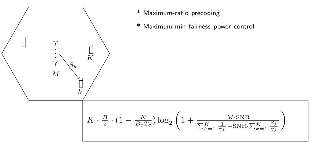
= bandwidth in Hertz (split equally between uplink and downlink)
  • $M$ = number of base station antennas
  • $K$ = number of multiplexed terminals
  • $B_c$ 
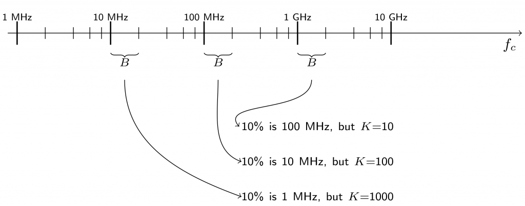
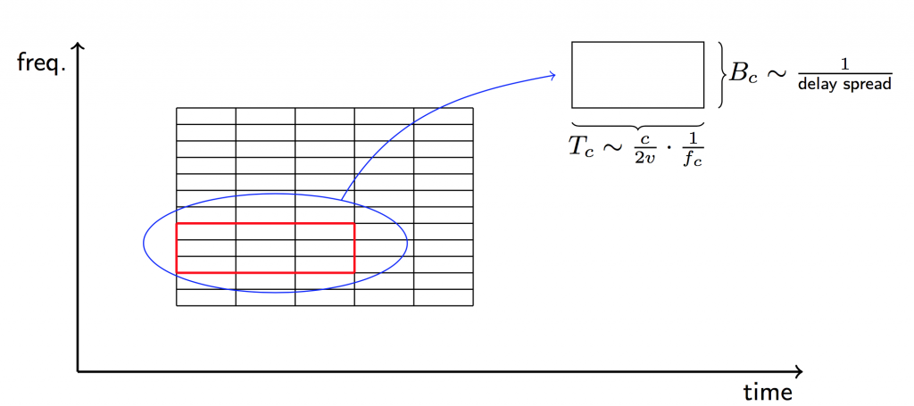
= coherence bandwidth in Hertz (independent of carrier frequency)
  • $T_c$ = coherence time in seconds (inversely proportional to carrier frequency)
  • SNR = signal-to-noise ratio (“normalized transmit power”)
  • $\beta_k$ = path loss for the k:th terminal
  • $\gamma_k$ = constant, close to $\beta_k$ with sufficient pilot power

This formula assumes independent Rayleigh fading, but the general conclusions remain under other models.

The factor that pre-multiplies the logarithm depends on $K$.
The pre-log factor is maximized when $K=B_c T_c/2$. The maximal value is $B B_c T_c/8$, which is proportional to $T_c$, and therefore proportional to the wavelength. Due to the multiplication $B T_c$, one can get same pre-log factor using a smaller bandwidth by instead increasing the wavelength, i.e., reducing the carrier frequency. At the same time, assuming appropriate scaling of the number of antennas, $M$, with the number of terminals, $K$, the quantity inside of the logarithm is a constant.

Concluding, the sum spectral efficiency (in b/s/Hz) easily can double for every doubling of the wavelength: a megahertz of bandwidth at 100 MHz carrier is ten times more worth than a megahertz of bandwidth at a 1 GHz carrier. So while there is more bandwidth available at higher carriers, the potential multiplexing gains are correspondingly smaller.

In this example,

all three setups give the same sum-throughput, however, the throughput per terminal is vastly different.

Summer School on Signal Processing for 5G

If you want to learn about signal processing foundations for Massive MIMO and mmWave communications, you should attend the

2017 Joint IEEE SPS and EURASIP Summer School on Signal Processing for 5G

Signal processing is at the core of the emerging fifth generation (5G) cellular communication systems, which will bring revolutionary changes to the physical layer. Unlike other 5G events, the objective of this summer school is to teach the main physical-layer techniques for 5G from a signal-processing perspective. The lectures will provide a background on the 5G wireless communication concepts and their formulation from a signal processing perspective. Emphasis will be placed on showing specifically how cutting-edge signal processing techniques can and will be applied to 5G. Keynote speeches by leading researchers from Ericsson, Huawei, China Mobile, and Volvo complement the technical lectures.

The summer school covers the following specific topics:

  • Massive MIMO communication in TDD and FDD
  • mmWave communications and compressed sensing
  • mmWave positioning
  • Wireless access for massive machine-type communications

The school takes place in Gothenburg, Sweden, from May 29th to June 1st, in the week after ICC in Paris.

This event belongs to the successful series of IEEE SPS and EURASIP Seasonal Schools in Signal Processing. The 2017 edition is jointly organized by Chalmers University of Technology, Linköping University, The University of Texas at Austin, Aalborg University and the University of Vigo.

Registration is now open. A limited number of student travel grants will be available.

For more information and detailed program, see: http://www.sp-for-5g.com/

Upside-Down World

The main track for 5G seems to be FDD for “old bands” below 3 GHz and TDD for “new bands” above 3 GHz (particularly mmWave frequencies). But physics advices us to the opposite:

  • At lower frequencies, larger areas are covered, thus most connections are likely to experience non-line-of-sight propagation. Since channel coherence is large (scales inverse proportionally to the Doppler), there is room for many terminals to transmit uplink pilots from which the base station consequently can obtain CSI. Reciprocity-based beamforming in TDD operation is scalable with respect to the number of base station antennas and delivers great value.
  • As the carrier frequency is increased, the coverage area shrinks; connections are more and more likely to experience line-of-sight propagation. At mmWave frequencies, all connections are either line-of-sight, or consist of a small number of reflected components. Then the channel can be parameterized with only few angular parameters; FDD operation with appropriate flavors of beam tracking may work satisfactorily. Reciprocity certainly would be desirable in this case too, but may not be necessary for the system to function.

Physics has given us the reciprocity principle. It should be exploited in wireless system design.