Contemporary base stations are equipped with analog-to-digital converters (ADCs) that take samples described by 12-16 bits. Since the communication bandwidth is up to 100 MHz in LTE Advanced, a sampling rate of a 500 Msample/s is quite sufficient for the ADC. The power consumption of such an ADC is at the order of 1 W. Hence, in a Massive MIMO base station with 100 antennas, the ADCs would consume around 100 W!

Fortunately, the 1600 bit/sample that are effectively produced by 100 16-bit ADCs are much more than what is needed to communicate at practical SINRs. For this reason, there is plenty of research on Massive MIMO base stations equipped with lower-resolution ADCs. The use of 1-bit ADCs has received particular attention. Some good paper references are provided in a previous blog post: Are 1-bit ADCs sufficient? While many early works considered narrowband channels, recent papers (e.g., Quantized massive MU-MIMO-OFDM uplink) have demonstrated that 1-bit ADCs can also be used in practical frequency-selective wideband channels. I’m impressed by the analytical depth of these papers, but I don’t think it is practically meaningful to use 1-bit ADCs.

Do we really need 1-bit ADCs?

I think the answer is no in most situations. The reason is that ADCs with a resolution of around 6 bits strike a much better balance between communication performance and power consumption. The state-of-the-art 6-bit ADCs are already very energy-efficient. For example, the paper “A 5.5mW 6b 5GS/S 4×-lnterleaved 3b/cycle SAR ADC in 65nm CMOS” from ISSCC 2015 describes a 6-bit ADC that consumes 5.5 mW and has a huge sampling rate of 5 Gsample/s, which is sufficient even for extreme mmWave applications with 1 GHz of bandwidth. In a base station equipped with 100 of these 6-bit ADCs, less than 1 W is consumed by the ADCs. That will likely be a negligible factor in the total power consumption of any base station, so what is the point in using a lower resolution than that?

The use of 1-bit ADCs comes with a substantial loss in communication rate. In contrast, there is a consensus that Massive MIMO with 3-5 bits per ADC performs very close to the unquantized case (see Paper 1, Paper 2, Paper 3, Paper 4, Paper 5). The same applies for 6-bit ADCs, which provide an additional margin that protects against strong interference. Note that there is nothing magical with 6-bit ADCs; maybe 5-bit or 7-bit ADCs will be even better, but I don’t think it is meaningful to use 1-bit ADCs.

Will 1-bit ADCs ever become useful?

To select a 1-bit ADC, instead of an ADC with higher resolution, the energy consumption of the receiving device must be extremely constrained. I don’t think that will ever be the case in base stations, because the power amplifiers are dominating their energy consumption. However, the case might be different for internet-of-things devices that are supposed to run for ten years on the same battery. To make 1-bit ADCs meaningful, we need to greatly simplify all the other hardware components as well. One potential approach is to make a dedicated spatial-temporal waveform design, as described in this paper.

This is supposedly a simple question to answer; an antenna is a device that emits radio waves. However, it is easy to get confused when comparing wireless communication systems with different number of transmit antennas, because these systems might use antennas with different physical sizes and properties. In fact, you can seldom find fair comparisons between contemporary single-antenna systems and Massive MIMO in the research literature.

Each antenna type has a predefined radiation pattern, which describes its inherent directivity; that is, how the gain of the emitted signal differs in different angular directions. An ideal isotropic antenna has no directivity, but a practical antenna always has a certain directivity, measured in dBi. For example, a half-wavelength dipole antenna has 2.15 dBi, which means that there is one angular direction in which the emitted signal is 2.15 dB stronger than it would be with a corresponding isotropic antenna. On the other hand, there are other angular directions in which the emitted signal is weaker. This is not a problem as long as there will not be any receivers in those directions.

In cellular communications, we are used to deploying large vertical antenna panels that cover a 120 degree horizontal sector and have a strong directivity of 15 dBi or more. Such a panel is made up of many small radiating elements, each having a directivity of a few dBi. By feeding them with the same input signal, a higher dBi is achieved for the panel. For example, if the panel consists of 8 patch antenna elements, each having 7 dBi, then you get a 7+10·log₁₀(8) = 16 dBi antenna.

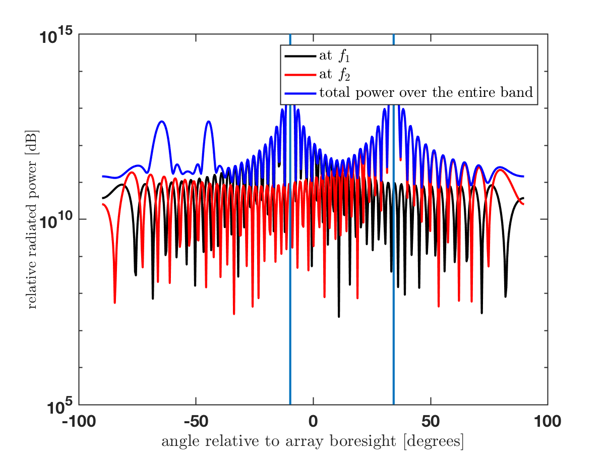
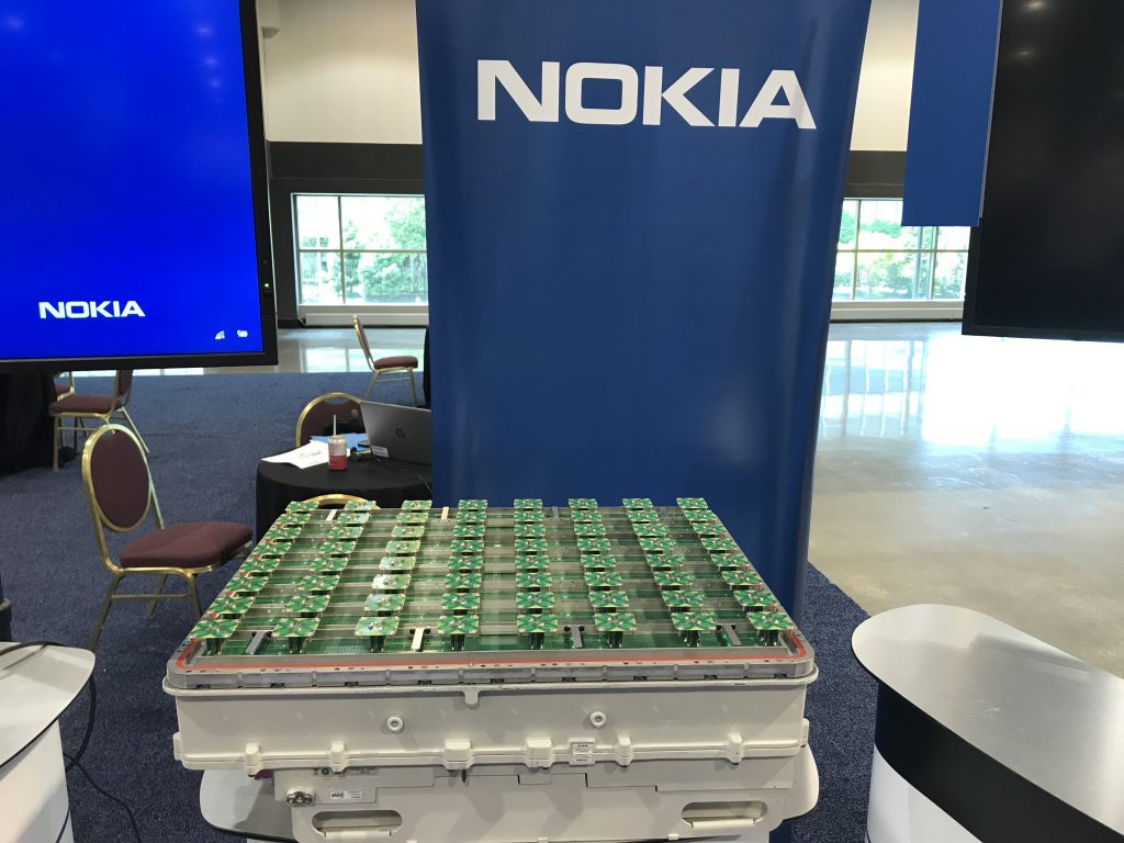
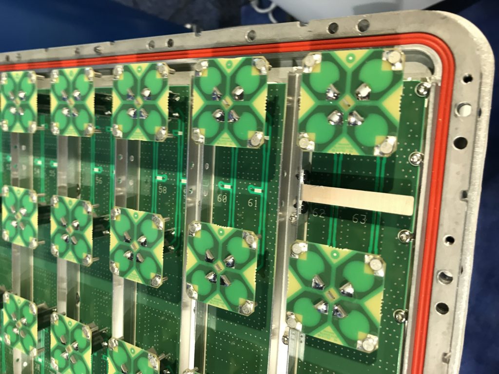
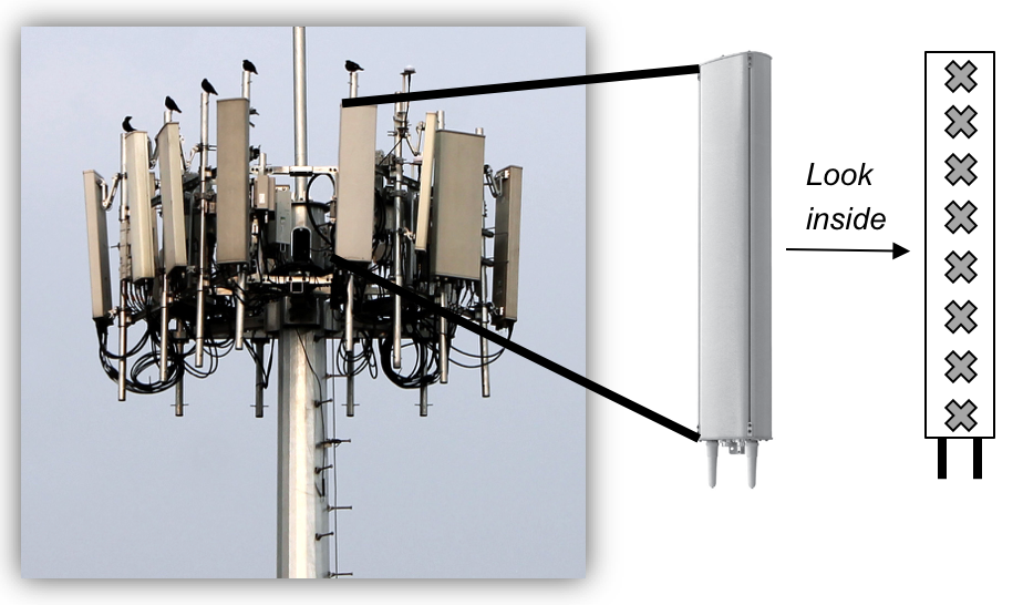
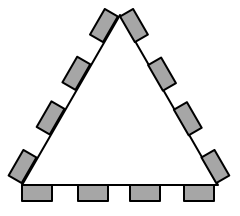
The picture above shows a real LTE site that I found in Nanjing, China, a couple of years ago. Looking at it from above, the site is structured as illustrated to the right. The site consists of three sectors, each containing a base station with four vertical panels. If you would look inside one of the panels, you will (probably) find 8 cross-polarized vertically stacked radiating elements, as illustrated in Figure 1. There are two RF input signals per panel, one per polarization, thus each panel acts as two antennas. This is how LTE with 8TX-sectors is deployed: 4 panels with dual polarization per base station.

At the exemplified LTE site, there is a total of 8·8·3 =192 radiating elements, but only 8·3 = 24 antennas. This disparity can lead to a lot of confusion. The Massive MIMO version of the exemplified LTE site may have the same form factor, but instead of 24 antennas with 16 dBi, you would have 192 antennas with 7 dBi. More precisely, you would connect each of the existing radiating elements to a separate RF input signal to create a larger number of antennas. Therefore, I suggest to use the following antenna definition from the book Massive MIMO Networks:

Note that, with this definition, an array that uses analog beamforming (e.g., a phased array) only constitutes one antenna. It is usually called an adaptive antenna since the radiation pattern can be changed over time, but it is nevertheless a single antenna. Massive MIMO for sub-6 GHz frequencies is all about adding RF chains (also known as antenna ports), while not necessarily adding more radiating elements than in a contemporary system.

What is the purpose of having more RF chains?

With more RF chains, you have more degrees of freedom to modify the radiation pattern of the transmitted signal based on where the receiver is located. When transmitting a precoded signal to a single user, you adjust the phases of the RF input signals to make them all combine constructively at the intended receiver.

The maximum antenna/array gain is the same when using one 16 dBi antenna and when using 8 antennas with 7 dBi. In the first case, the radiation pattern is usually static and thus only a line-of-sight user located in the center of the cell sector will obtain this gain. However, if the antenna is adaptive (i.e., supports analog beamforming), the main lobe of the radiation pattern can be also steered towards line-of-sight users located in other angular directions. This feature might be sufficient for supporting the intended single-user use-cases of mm-wave technology (see Figure 4 in this paper).

In contrast, in the second case, we can adjust the radiation pattern by 8-antenna precoding to deliver the maximum gain to any user in the sector. This feature is particularly important for non-line-of-sight users (e.g., indoor use-cases), for which the signals from the different radiating elements will likely be received with “random” phase shifts and therefore add non-constructively, unless we compensate for the phases by digital precoding.

Note that most papers on Massive MIMO keep the antenna gain constant when comparing systems with different number of antennas. There is nothing wrong with doing that, but one cannot interpret the single-antenna case in such a study as a contemporary system.

Another, perhaps more important, feature of having multiple RF chains is that we can spatially multiplex several users when having multiple antennas. For this you need at least as many RF inputs as there are users. Each of them can get the full array gain and the digital precoding can be also used to avoid inter-user interference.