2018 was the year when the deployment of Massive MIMO capable base stations began in many countries, such as Russia and USA. Nevertheless, I still see people claiming that Massive MIMO is “too expensive to implement“. In fact, this particular quote is from a review of one of my papers that I received in November 2018. It might have been an accurate (but pessimistic) claim a few years ago, but nowadays it is plainly wrong.
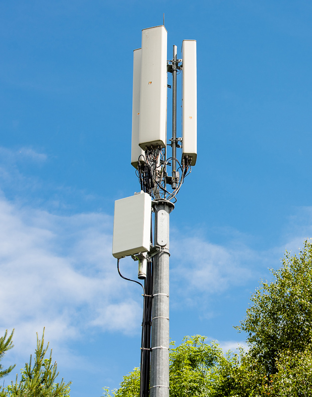
This photo is from the Bristol Temple Meads railway station. The Massive MIMO panel is at the bottom. (Photo: Vodafone UK Media Centre.)
I recently came across a website about telecommunication infrastructure by Peter Clarke. He has gathered photos of Massive MIMO antenna panels that have been deployed by Vodafone and by O2 in the United Kingdom. These deployments are using hardware from Huawei and Nokia, respectively. Their panels have similar form factors and are rather easy to recognize in the pictures since they are almost square-shaped, as compared to conventional rectangular antenna panels. You can see the difference in the image to the right. The technology used in these panels are probably similar to the Ericsson panel that I have previously written about. I hope that as many wireless communication researchers as possible will see these images and understand that Massive MIMO is not too expensive to implement but has in fact already been deployed in commercial networks.
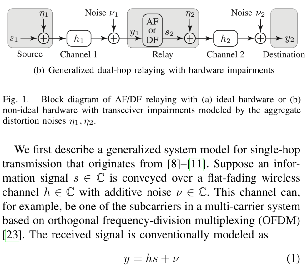
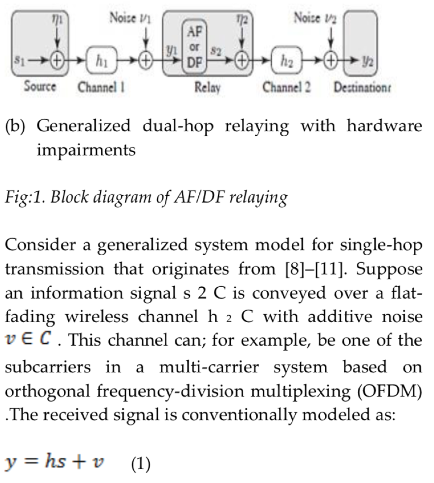
I was asked to review my ownpapers three times during 2018. Or more precisely, I was asked to review papers by other people that contain the same content as some of my most well-cited papers. The review requests didn’t come from IEEE journals but less reputed journals. However, the papers were still written in such a way that they would likely pass through the automatic plagiarism detection systems that IEEE, EDAS, and others are using. How is that possible? Here is an example of how it could look like.
Original:
Plagiarized version:
As you can see, the authors are using the same equations and images, but the sentences are slightly paraphrased and the inline math is messed up. The meanings of the sentences are the same, but the different wording might be enough to pass through a plagiarism detection system that compares the words in different documents without being able of understanding the context. (I have better examples of this than the one shown above, but I didn’t want to reveal myself as a reviewer of those papers.)
This approach to plagiarism is known as rogeting and basically means that you replace words in the original text with synonyms from a thesaurus with the purpose of fooling plagiarism detection systems. There are already online tools that can do this, often resulting unnatural sentence structures, but the advances in deep learning and natural language processing will probably help to refine these tools in the near future.
Is this an increasing problem?
This is hard to tell, but there are definitely indications in that direction. The reason might be that digital technology has made it easier to plagiarize. If you want to plagiarize a scientific paper, you don’t need to retype every word by hand. You can simply download the LaTeX code of the paper from ArXiV.org (everything that an author uploads can be downloaded by others) and simply change the author names and then hide your misconduct by rogeting.
On the other hand, plagiarism detection systems are also becoming more sophisticated over time. My point is that we should never trust these systems as being reliable because people will always find ways to fool them. The three plagiarized papers that I detected in 2018 were all submitted to less reputed journals, but they apparently had a functioning peer-review system where researchers like me could spot the similarities despite the rogeting. Unfortunately, there are plenty of predatory journals and conferences that might not have any peer-review whatsoever and will publish anything if you just pay them to do so.
Does anyone benefit from plagiarism?
I am certainly annoyed by the fact that some people have the dishonesty to steal other people’s research and pretend that it is their research. At the same time, I’m wondering if anyone really benefits from doing that? The predatory journals make money from it, but what is in it for the authors? Whenever I review the CV of someone that applies for a position in my group, I have a close look at their list of publications. If it only contains papers published in unknown journals and conferences, I treat it as if the person has no real publications. I might even regard it as more negative to have such publications in the CV than to have no publications at all! I suppose that many other professors do the same thing, and I truly hope that recruiters at companies also have the skills of evaluating publication lists. Having published in a predatory journal must be viewed as a big red flag!
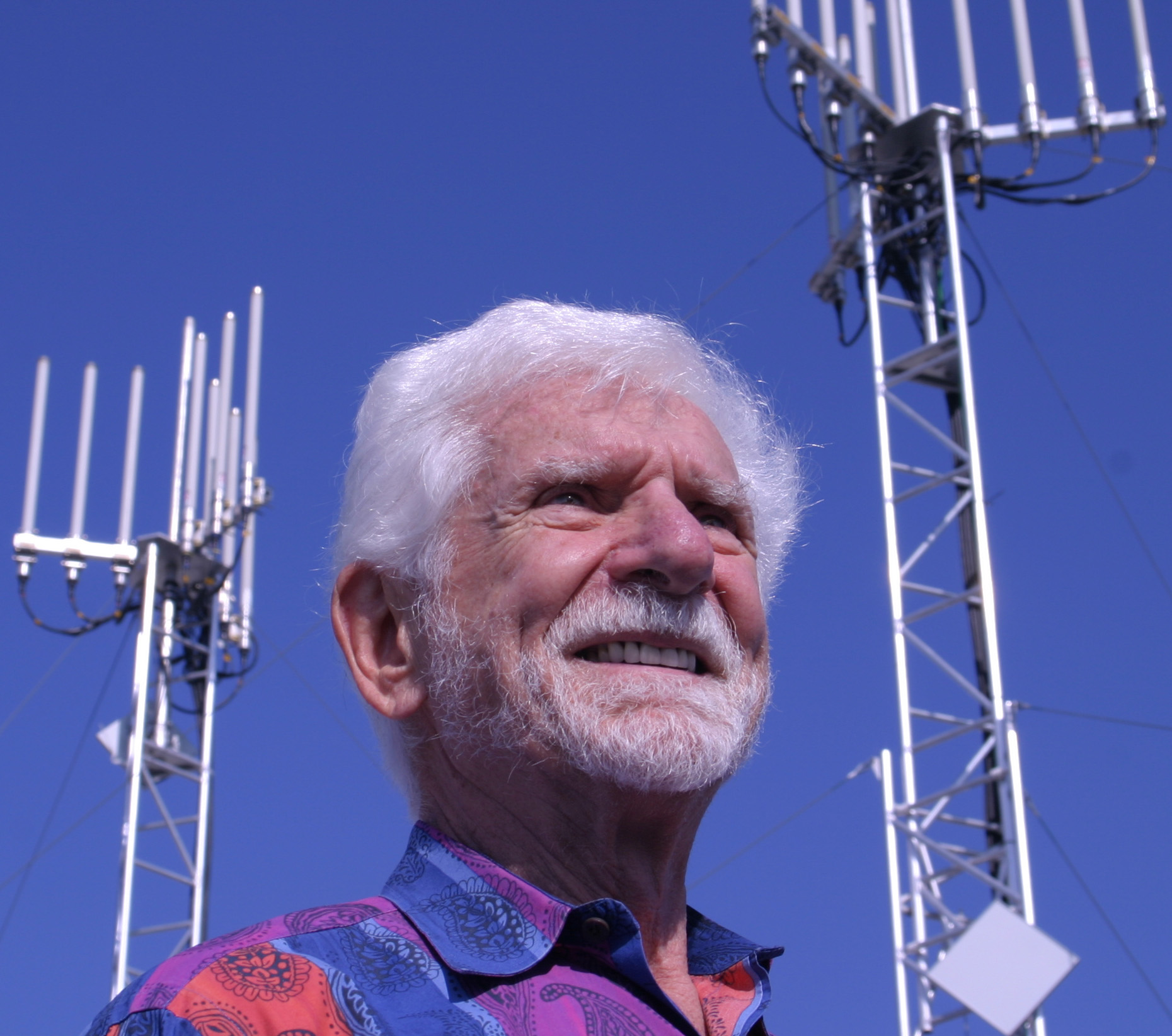
I found an interesting news article by Reily Gregson where he is interviewing Martin Cooper, who is considered the father of the handheld cell phone. Cooper is talking about spatial division multiple access, the early name of the multi-user MIMO technology, and how “computers weren’t powerful enough to operate it” at the time it was invented at his startup-company ArrayComm.
Cooper points out that “Today we spray energy in all directions. Why not aim it directly?” He then provides three examples of why multi-user MIMO solves important practical problems:
“First, deploying cellular and derivative technologies is costly. Second, the quality of wireless communicating must be comparable or better than that of wireline in order to compete with wireline, said Cooper. And as spectrum is finite, technology must work toward greater efficiency.”
Furthermore, he says that ArrayComm’s multi-user MIMO solution “requires fewer base stations, which cuts costs. The technology also is adaptive, which simplifies network design and reduces site acquisition and installation costs.”
By the way, did I forgot to say that this interview is from 1996…?
I explained in a previous blog post why the efforts to commercialize multi-user MIMO in the nineties were not as successful as Cooper and others might have hoped for. Now, more than 20 years later, we are about to witness a large-scale deployment of 5G technology, in which MIMO is a key component. The industry has hopefully learned from the negative past experiences when Massive MIMO is now being deployed in commercial networks. One thing we know for sure is that computational complexity is not a problem anymore.
Adaptive beamforming for wireless communications has a long history, with the modern research dating back to the 70s and 80s. There is even a paper from 1919 that describes the development of directive transatlantic communication practices that were developed during the First World War. Many of the beamforming methods that are considered today can be found already in the magazine paper Beamforming: A Versatile Approach to Spatial Filtering from 1988. Plenty of further work was carried out in the 90s and 00s, before the Massive MIMO paradigm.
I think it is fair to say that no fundamentally new beamforming methods have been developed in the Massive MIMO literature, but we have rather taken known methods and generalized them to take imperfect channel state information and other practical aspects into account. And then we have developed rigorous ways to quantify the achievable rates that these beamforming methods achieve and studied the asymptotic behaviors when having many antennas. Closed-form expressions are available in some special cases, while Monte Carlo simulations can be used to compute these expressions in other cases.
As beamforming has evolved from an analog phased-array concept, where angular beams are studied, to a digital concept where the beamforming is represented in multi-dimensional vector spaces, it easy to forget the basic properties of array processing. That is why we dedicated Section 7.4 in Massive MIMO Networks to describe how the physical beam width and spatial resolution depend on the array geometry.
In particular, I’ve observed a lot of confusion about the dimensionality of MIMO arrays, which are probably rooted in the confusion around the difference between an antenna (which is something connected to an RF chain) and a radiating element. I explained this in detail in a previous blog post and then exemplified it based on a recent press release. I have also recorded the following video to visually explain these basic properties:
A recent white paper from Ericsson is also providing a good description of these concepts, particularly focused on how an array with a given geometry can be implemented with different numbers of RF chains (i.e., different numbers of antennas) depending on the deployment scenario. While having as many antennas as radiating element is preferable from a performance perspective, but the Ericsson researchers are arguing that one can get away with fewer antennas in the vertical direction in deployments where it is anyway very hard to resolve users in the elevation dimension.
“Open science is just science done right” is a quote from Prof. Jon Tennant in a recent podcast. He is referring to the movement away from the conventionally closed science community where you need to pay to gain access to research results and everyone treats data and simulation code as confidential. Since many funding agencies are requiring open access publishing and open data nowadays, we are definitely moving in the open science direction. But different research fields are at different positions on the scale between fully open and entirely closed science. The machine learning community has embraced open science to a large extent, maybe because the research requires common data sets. When the Nature Machine Intelligence journal was founded, more 3000 researchers signed a petition against its closed access and author fees and promised to not publish in that journal. However, research fields that for decades have been dominated by a few high-impact journals (such as Nature) have not reached as far.
IEEE is the main publisher of Massive MIMO research and has, fortunately, been quite liberal in terms of allowing for parallel publishing. At the time of writing this blog post, the IEEE policy is that an author is allowed to upload the accepted version of their paper on the personal website, the author’s employer’s website, and on arXiv.org. It is more questionable if it is allowed to upload papers in other popular repositories such as ResearchGate – can the ResearchGate profile pages count as personal websites?
It is we as researchers that need to take the steps towards open science. The publishers will only help us under the constraint that they can sustain their profits. For example, IEEE Access was created to have an open access alternative to the traditional IEEE journals, but its quality is no better than non-IEEE journals that have offered open access for a long time. I have published several papers in IEEE Access and although I’m sure that these papers are of good quality, I’ve been quite embarrassed by the poor review processes.
Personally, I try to make all my papers available on arXiv.org and also publish simulation code and data on my GitHub whenever I can, in an effort to support research reproducibility. My reasons for doing this are explained in the following video:
The tedious, time-consuming, and buggy nature of system-level simulations is exacerbated with massive MIMO. This post offers some relieve in the form of analytical expressions for downlink conjugate beamforming [1]. These expressions enable the testing and calibration of simulators—say to determine how many cells are needed to represent an infinitely large network with some desired accuracy. The trick that makes the analysis feasible is to let the shadowing grow strong, yet the ensuing expressions capture very well the behaviors with practical shadowings.
The setting is an infinitely large cellular network where each -antenna base station (BS) serves single-antenna users. The large-scale channel gains include pathloss with exponent and shadowing having log-scale standard deviation , with the gain between the th BS and the th user served by a BS of interest denoted by .With conjugate beamforming and receivers reliant on channel hardening, the signal-to-interference ratio (SIR) at such user is [2]
where is the gain from the serving BS and is the share of that BS’s power allocated to user . Two power allocations can be analyzed:
Uniform: .
SIR-equalizing [3]: , with the proportionality constant ensuring that . This makes . Moreover, as and grow large,
The analysis is conducted for , which makes it valid for arbitrary BS locations.
SIR
For notational compactness, let . Define as the solution to where is the lower incomplete gamma function. For , in particular, . Under a uniform power allocation, the CDF of is available in an explicit form involving the Gauss hypergeometric function (available in MATLAB and Mathematica):
where “” indicates asymptotic () equality, is such that the CDF is continuous, and
Alternatively, the CDF can be obtained by solving (e.g., with Mathematica) a single integral involving the Kummer function :
This latter solution can be modified for the SIR-equalizing power allocation as
Spectral Efficiency
The spectral efficiency of user is with CDF readily characterizable from the expressions given earlier. From , the sum spectral efficiency at the BS of interest can be found as Expressions for the averages and are further available in the form of single integrals.
With a uniform power allocation,
(1)
and . For the special case of , the Kummer function simplifies giving
(2)
With an equal-SIR power allocation
(3)
and .
Application to Relevant Networks
Let us now contrast the analytical expressions (computable instantaneously and exactly, and valid for arbitrary topologies, but asymptotic in the shadowing strength) with some Monte-Carlo simulations (lengthy, noisy, and bug-prone, but for precise shadowing strengths and topologies).
First, we simulate a 500-cell hexagonal lattice with , and . Figs. 1a-1b compare the simulations for – dB with the analysis. The behaviors with these typical outdoor values of are well represented by the analysis and, as it turns out, in rigidly homogeneous networks such as this one is where the gap is largest.
Figure 1: Analysis vs hexagonal network simulations with lognormal shadowing
For a more irregular deployment, let us next consider a network whose BSs are uniformly distributed. BSs (500 on average) are dropped around a central one of interest. For each network snapshot, users are then uniformly dropped until of them are served by the central BS. As before, , and . Figs. 2a-2b compare the simulations for dB with the analysis, and the agreement is now complete. The simulated average spectral efficiency with a uniform power allocation is b/s/Hz/user while (2) gives b/s/Hz/user.
Figure 2: Analysis vs Poisson network simulations with lognornmal shadowing.
The analysis presented in this post is not without limitations, chiefly the absence of noise and pilot contamination. However, as argued in [1], there is a broad operating range (– with very conservative premises) where these effects are rather minor, and the analysis is hence applicable.
The University of Bristol continues to be one of the driving forces in demonstrating reciprocity-based Massive MIMO in time-division duplex. The two videos below are from an outdoor demo that was carried out in Bristol in March 2018. A 128-antenna testbed with a rectangular array of 4 rows and 32 single-polarized antennas per row were used. The demo was carried out with a carrier frequency of 3.5 GHz and featured spatial multiplexing of video streaming to 12 users.


 -antenna base station (BS) serves
  single-antenna users. The large-scale channel gains include pathloss with exponent
  and shadowing having log-scale standard deviation
  , with the gain between the
  th BS and the
  th user served by a BS of interest denoted by
  .
.
 is the gain from the serving BS and
  is the share of that BS’s power allocated to user
  .
. , with the proportionality constant ensuring that
  . This makes
  . Moreover, as
 , which makes it valid for arbitrary BS locations.
 . Define
  as the solution to
  where
where  is the lower incomplete gamma function. For
  , in particular,
  . Under a uniform power allocation, the CDF of
  is available in an explicit form involving the Gauss hypergeometric function
  (available in MATLAB and Mathematica):
 ” indicates asymptotic (
 ) equality,
  is such that the CDF is continuous, and
 :
:

 with CDF
  readily characterizable from the expressions given earlier. From
  , the sum spectral efficiency at the BS of interest can be found as
  Expressions for the averages
 ![\bar{C} = \mathbb{E} \big[ C_k \big]](http://ma-mimo.ellintech.se/wp-content/ql-cache/quicklatex.com-a887caab28778e8d91a237bcc86a9f3e_l3.png "Rendered by QuickLaTeX.com") and
and ![\bar{C}_{\scriptscriptstyle \Sigma} = \mathbb{E} \! \left[ C_{\scriptscriptstyle \Sigma} \right]](http://ma-mimo.ellintech.se/wp-content/ql-cache/quicklatex.com-865de5351a43ee6f0405ddb531ed84ee_l3.png "Rendered by QuickLaTeX.com") are further available in the form of single integrals.
are further available in the form of single integrals.
 . For the special case of

 ,
,  and
and  –
– dB with the analysis. The behaviors with these typical outdoor values of
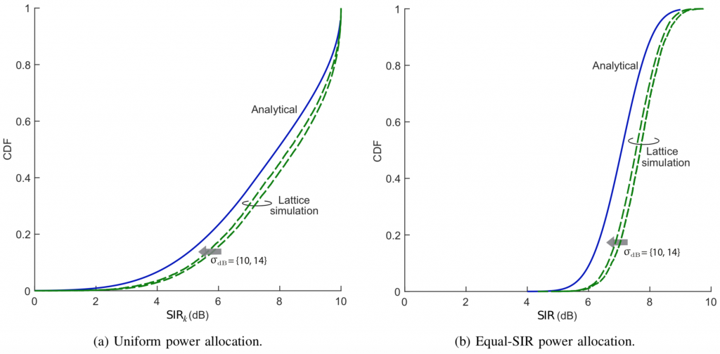
 and
and  . Figs. 2a-2b compare the simulations for
  dB with the analysis, and the agreement is now complete. The simulated average spectral efficiency with a uniform power allocation is
  b/s/Hz/user while (2) gives
  b/s/Hz/user.
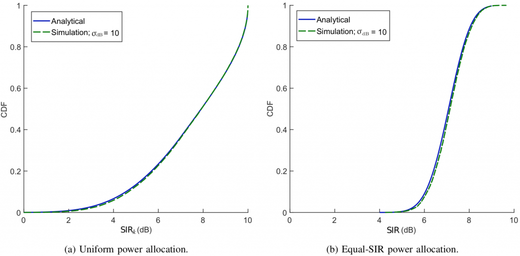
 –
– with very conservative premises) where these effects are rather minor, and the analysis is hence applicable.