The object of the competition is to design and train an algorithm that can determine the position of a user, based on estimated channel frequency responses between the user and an antenna array. Possible solutions may build on classic algorithms (fingerprinting, interpolation) or machine-learning approaches. Channel vectors from a dataset created with a MIMO channel sounder will be used.
Competing teams should present a poster at the conference, describing their algorithms and experiments.
A $500 USD prize will be awarded to the winning team.
Come listen to Liesbet Van der Perre, Professor at KU Leuven (Belgium) on Monday February 18 at 2.00 pm EST.
She gives a webinar on state-of-the-art circuit implementations of Massive MIMO, and outlines future research challenges. The webinar is based on, among others, this paper.
In more detail the webinar will summarize the fundamental technical contributions to efficient digital signal processing for Massive MIMO. The opportunities and constraints on operating on low-complexity RF and analog hardware chains are clarified. It will explain how terminals can benefit from improved energy efficiency. The status of technology and real-life prototypes will be discussed. Open challenges and directions for future research are suggested.
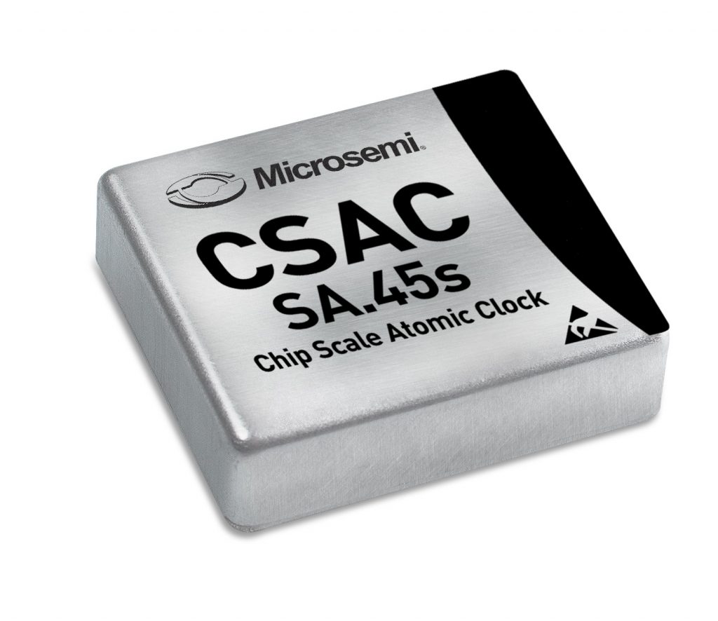
This chip-scale atomic clock (CSAC) device, developed by Microsemi, brings atomic clock timing accuracy (see the specs available in the link) in a volume comparable to a matchbox, and 120 mW power consumption. This is way too much for a handheld gadget, but undoubtedly negligible for any fixed installation powered from the grid. An alternative to synchronization through GNSS that works anywhere, including indoor in GNSS-denied environments.
I haven’t seen a list price, and I don’t know how much exotic metals and what licensing costs that its manufacture requires, but let’s ponder the possibility that a CSAC could be manufactured for the mass-market for a few dollars each. What new applications would then become viable in wireless?
The answer is mostly (or entirely) speculation. One potential application that might become more practical is positioning using distributed arrays. Another is distributed multipair relaying. Here and here are some specific ideas that are communication-theoretically beautiful, and probably powerful, but that seem to be perceived as unrealistic because of synchronization requirements. Perhaps CoMP and distributed MIMO, a.k.a. “cell-free Massive MIMO”, applications could also benefit.
Other applications might be applications for example in IoT, where a device only sporadically transmits information and wants to stay synchronized (perhaps there is no downlink, hence no way of reliably obtaining synchronization information). If a timing offset (or frequency offset for that matter) is unknown but constant over a very long time, it may be treated as a deterministic unknown and estimated. The difficulty with unknown time and frequency offsets is not their existence per se, but the fact that they change quickly over time.
It’s often said (and true) that the “low” speed of light is the main limiting factor in wireless. (Because channel state information is the main limiting factor of wireless communications. If light were faster, then channel coherence would be longer, so acquiring channel state information would be easier.) But maybe the unavailability of a ubiquitous, reliable time reference is another, almost as important, limiting factor. Can CSAC technology change that? I don’t know, but perhaps we ought to take a closer look.
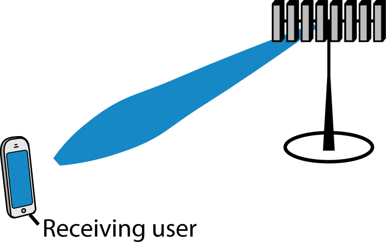
When an antenna array is used to focus a transmitted signal on a receiver, we call this beamforming (or precoding) and we usually illustrate it as shown to the right. This cartoonish illustration is only applicable when the antennas are gathered in a compact array and there is a line-of-sight channel to the receiver.
If we want to deploy very many antennas, as in Massive MIMO, it might be preferable to distribute the antennas over a larger area. One such deployment concept is called Cell-free Massive MIMO. The basic idea is to have many distributed antennas that are transmitting phase-coherently to the receiving user. In other words, the antennas’ signal components add constructively at the location of the user, just as when using a compact array for beamforming. It is therefore convenient to call it beamforming in both cases—algorithmically it is the same thing!
The question is: How can we illustrate the beamforming effect when using a distributed array?
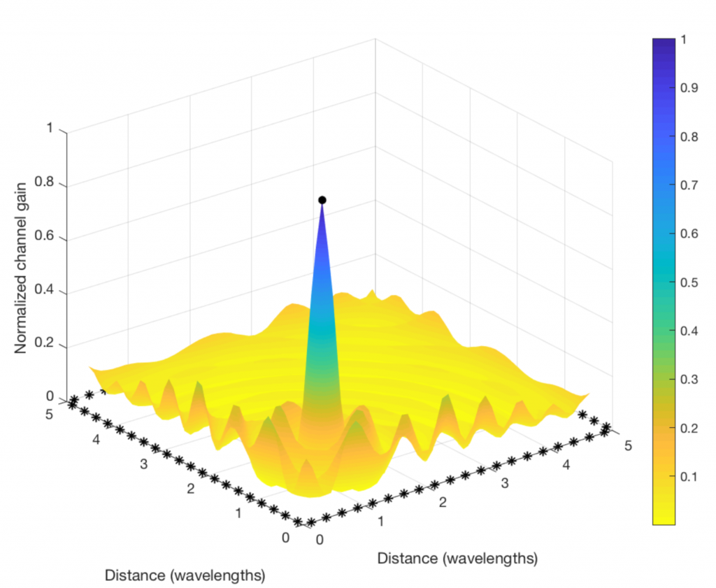
The figure below shows how to do it. I consider a toy example with 80 star-marked antennas deployed along the sides of a square and these antennas are transmitting sinusoids with equal power, but different phases. The phases are selected to make the 80 sine-components phase-aligned at one particular point in space (where the receiving user is supposed to be):
Clearly, the “beamforming” from a distributed array does not give rise to a concentrated signal beam, but the signal amplification is confined to a small spatial region (where the color is blue and the values on the vertical axis are close to one). This is where the signal components from all the antennas are coherently combined. There are minor fluctuations in channel gain at other places, but the general trend is that the components are non-coherently combined everywhere except at the receiving user. (Roughly the same will happen in a rich multipath channel, even if a compact array is used for transmission.)
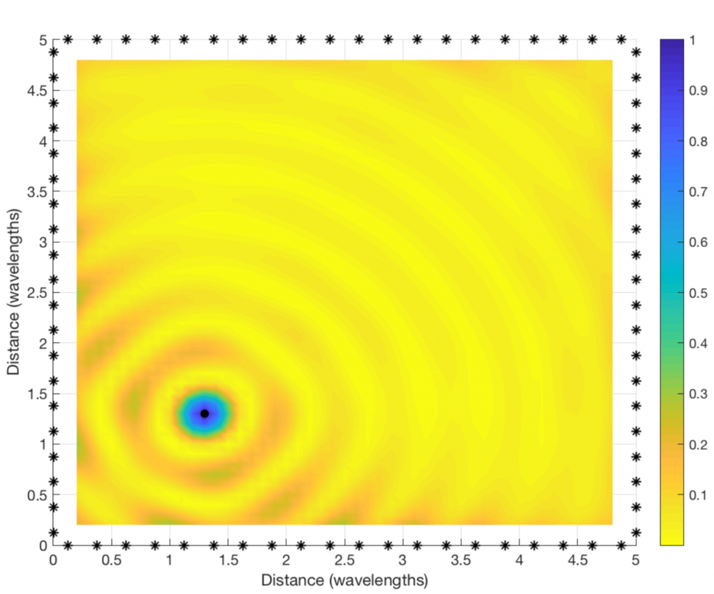
By looking at a two-dimensional version of the figure (see below), we can see that the coherent combination occurs in a circular region that is roughly half a wavelength in diameter. At the carrier frequencies used for cellular networks, this region will only be a few centimeters or millimeters wide. It is almost magical how this distributed array can amplify the signal at such a tiny spatial region! This spatial region is probably what the company Artemis is calling a personal cell (pCell) when marketing their distributed MIMO solution.
If you are into the details, you might wonder why I simulated a square region that is only a few wavelengths wide, and why the antenna spacing is only a quarter of a wavelength. This assumption was only made for illustrative purposes. If the physical antenna locations are fixed but we would reduce the wavelength, the size of the circular region will reduce and the ripples will be more frequent. Hence, we would need to compute the channel gain at many more spatial sample points to produce a smooth plot.
Reproduce the results: The code that was used to produce the plots can be downloaded from my GitHub.
Although there are nowadays many Massive MIMO testbeds around the world, there are very few open datasets with channel measurement results. This will likely change over the next few years, spurred by the need for having common datasets when applying and evaluating machine learning methods in wireless communications.
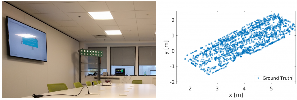
The Networked Systems group at KU Leuven has recently made the results from one of their measurement campaigns openly available. It includes 36 user positions and two base station configurations: one 64-antenna co-located array and one distributed deployment with two 32-antenna arrays.
The following video showcases the measurement setup:
The tedious, time-consuming, and buggy nature of system-level simulations is exacerbated with massive MIMO. This post offers some relieve in the form of analytical expressions for downlink conjugate beamforming [1]. These expressions enable the testing and calibration of simulators—say to determine how many cells are needed to represent an infinitely large network with some desired accuracy. The trick that makes the analysis feasible is to let the shadowing grow strong, yet the ensuing expressions capture very well the behaviors with practical shadowings.
The setting is an infinitely large cellular network where each -antenna base station (BS) serves single-antenna users. The large-scale channel gains include pathloss with exponent and shadowing having log-scale standard deviation , with the gain between the th BS and the th user served by a BS of interest denoted by .With conjugate beamforming and receivers reliant on channel hardening, the signal-to-interference ratio (SIR) at such user is [2]
where is the gain from the serving BS and is the share of that BS’s power allocated to user . Two power allocations can be analyzed:
Uniform: .
SIR-equalizing [3]: , with the proportionality constant ensuring that . This makes . Moreover, as and grow large,
The analysis is conducted for , which makes it valid for arbitrary BS locations.
SIR
For notational compactness, let . Define as the solution to where is the lower incomplete gamma function. For , in particular, . Under a uniform power allocation, the CDF of is available in an explicit form involving the Gauss hypergeometric function (available in MATLAB and Mathematica):
where “” indicates asymptotic () equality, is such that the CDF is continuous, and
Alternatively, the CDF can be obtained by solving (e.g., with Mathematica) a single integral involving the Kummer function :
This latter solution can be modified for the SIR-equalizing power allocation as
Spectral Efficiency
The spectral efficiency of user is with CDF readily characterizable from the expressions given earlier. From , the sum spectral efficiency at the BS of interest can be found as Expressions for the averages and are further available in the form of single integrals.
With a uniform power allocation,
(1)
and . For the special case of , the Kummer function simplifies giving
(2)
With an equal-SIR power allocation
(3)
and .
Application to Relevant Networks
Let us now contrast the analytical expressions (computable instantaneously and exactly, and valid for arbitrary topologies, but asymptotic in the shadowing strength) with some Monte-Carlo simulations (lengthy, noisy, and bug-prone, but for precise shadowing strengths and topologies).
First, we simulate a 500-cell hexagonal lattice with , and . Figs. 1a-1b compare the simulations for – dB with the analysis. The behaviors with these typical outdoor values of are well represented by the analysis and, as it turns out, in rigidly homogeneous networks such as this one is where the gap is largest.
Figure 1: Analysis vs hexagonal network simulations with lognormal shadowing
For a more irregular deployment, let us next consider a network whose BSs are uniformly distributed. BSs (500 on average) are dropped around a central one of interest. For each network snapshot, users are then uniformly dropped until of them are served by the central BS. As before, , and . Figs. 2a-2b compare the simulations for dB with the analysis, and the agreement is now complete. The simulated average spectral efficiency with a uniform power allocation is b/s/Hz/user while (2) gives b/s/Hz/user.
Figure 2: Analysis vs Poisson network simulations with lognornmal shadowing.
The analysis presented in this post is not without limitations, chiefly the absence of noise and pilot contamination. However, as argued in [1], there is a broad operating range (– with very conservative premises) where these effects are rather minor, and the analysis is hence applicable.
Drones could shape the future of technology, especially if provided with reliable command and control (C&C) channels for safe and autonomous flying, and high-throughput links for multi-purpose live video streaming. Some months ago, Prabhu Chandhar’s guest post discussed the advantages of using massive MIMO to serve drone – or unmanned aerial vehicle (UAV) – users. More recently, our Paper 1 and Paper 2 have quantified such advantages under the realistic network conditions specified by the 3GPP. While demonstrating that massive MIMO is instrumental in enabling support for UAV users, our works also show that merely upgrading existing base stations (BS) with massive MIMO might not be enough to provide a reliable service at all UAV flying heights. Indeed, hardware solutions need to be complemented with signal processing enhancements through all communications phases, namely, 1) UAV cell selection and association, 2) downlink BS-to-UAV transmissions, and 3) uplink UAV-to-BS transmissions. These are outlined below.
1. UAV cell selection and association
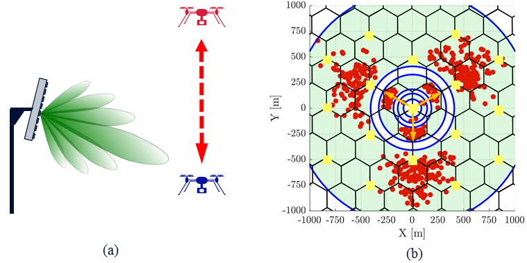
As depicted in Figure 1(a), most existing cellular BSs create a fixed beampattern towards the ground. Thanks to this, ground users tend to perceive a strong signal strength from nearby BSs, which they use for connecting to the network. Instead, aerial users such as the red drone in Figure 1(a) only receive weak sidelobe-generated signals from a nearby BS when flying above it. This results in a deployment planning issue as illustrated in Figure 1(b), where due to the radiation of a strong sidelobe, the tri-sector BSs located in the origin can be the preferred server for far-flung UAVs (red spots). Consequently, these UAVs might experience strong interference, since they perceive signals from a multiplicity of BSs with similar power.
Figure 1. (a) Illustration of a downtilted cellular BS and its beampattern: low (blue) UAV receives strong main lobe signals, whereas high (red) drone only receives weak sidelobe-generated signals. (b) 150-meter-high UAVs (red dots) associated with a three-cell BS site located at the origin and pointing at 30°, 150°, and 270°. The three BSs of each cellular site (orange squares) generate ground cells represented by hexagons.
On the other hand, thanks to their capability of beamforming the synchronization signals used for user association, massive MIMO systems ensure that aerial users generally connect to a nearby BS. This optimized association enhances the robustness of the mobility procedures, as well as the downlink and uplink data phases.
2. Downlink BS-to-UAV transmissions
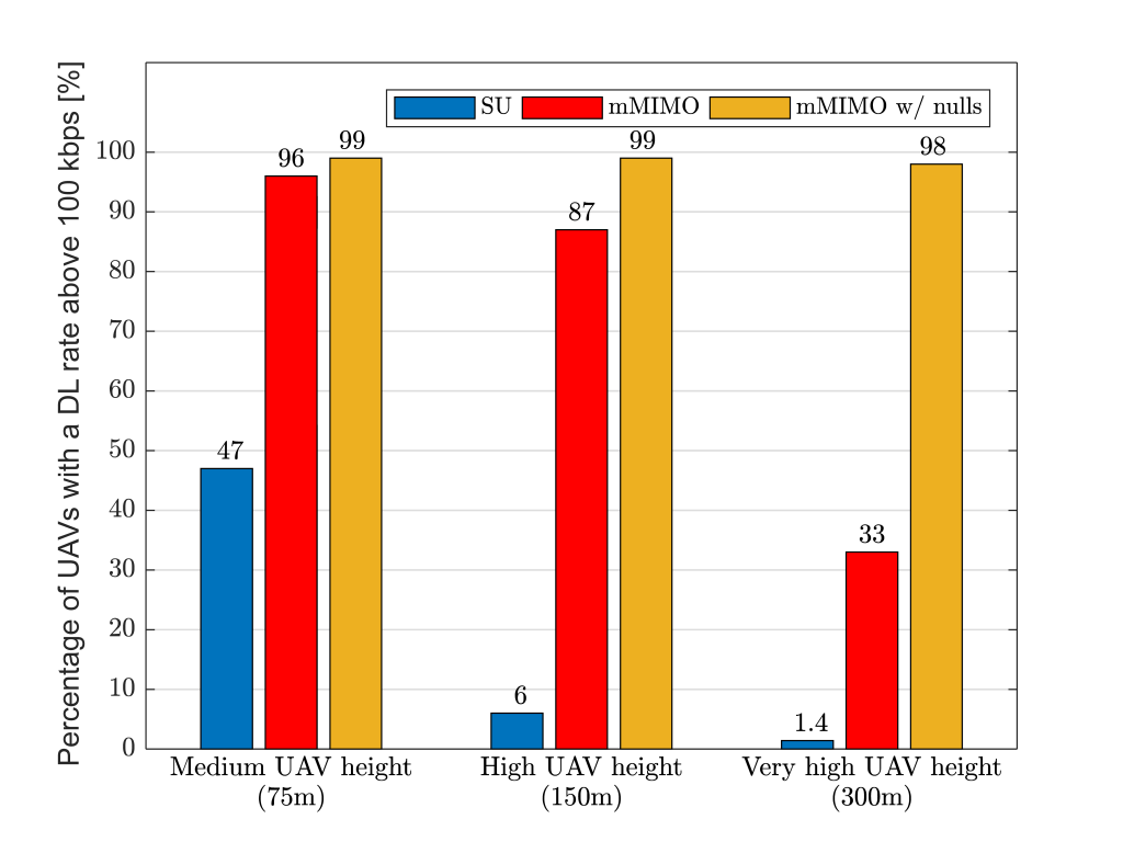
During the downlink data phase, UAV users are very sensitive to the strong inter-cell interference generated from a plurality of BSs, which are likely to be in line-of-sight. This may result in performance degradation, preventing UAVs from receiving critical C&C information, which has an approximate rate requirement of 60-100 kbps. Indeed, Figure 2 shows how conventional cellular networks (‘SU’) can only guarantee 100 kbps to a mere 6% of the UAVs flying at 150 meters. A conventional massive MIMO system (‘mMIMO’) enhances the data rates, albeit only 33% of the UAVs reach 100 kbps when they fly at 300 meters. This is due to a well-known effect: pilot contamination. Such an effect is particularly severe in scenarios with UAV users, since they can create strong uplink interference to many line-of-sight BSs simultaneously. In contrast, the pilot contamination decays much faster with distance for ground UEs.
In a nutshell, Figure 2 tells us that complementing conventional massive MIMO with explicit inter-cell interference suppression (‘mMIMO w/ nulls’) is essential when supporting high UAVs. In a ‘mMIMO w/ nulls’ system, BSs incorporate additional signal processing features that enable them to perform a twofold task. First, leveraging channel directionality, BSs can spatially separate non-orthogonal pilots transmitted by different UAVs. Second, by dedicating a certain number of spatial degrees of freedom to place radiation nulls, BSs can mitigate interference on the directions corresponding to users in other cells that are most vulnerable to the BS’s interference. Indeed, these additional capabilities dramatically increase the percentage of UAVs that meet the 100 kbps requirement when these are flying at 300 m, from 33% (‘mMIMO’) to a whopping 98% (‘mMIMO w/ nulls’).
Figure 2. Percentage of UAVs with a downlink C&C rate above 100 kbps for three representative UAV heights. ‘SU’ denotes a conventional cellular network with a single antenna port, ‘mMIMO’ represents a system with 8×8 dual-polarized antenna arrays and 128 antenna ports, and ‘mMIMO w/ nulls’ complements the latter with additional space-domain inter-cell interference suppression techniques.
3. Uplink UAV-to-BS transmissions
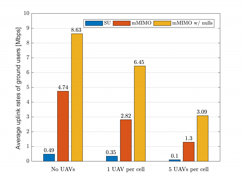
Unlike the downlink, where UAVs should be protected to prevent a significant performance degradation, it is the ground users who we should care about in the uplink. This is because line-of-sight UAVs can generate strong interference towards many BSs, therefore overwhelming the weaker signals transmitted by non-line-of-sight ground users. The consequences of such a phenomenon are illustrated in Figure 3, where the uplink rates of ground users plummet as the number of UAVs increases.
Again, ‘mMIMO w/nulls’ – incorporating additional space-domain inter-cell interference suppression capabilities – can solve the above issue and guarantee a better performance for legacy ground users.
Figure 3. Average uplink rates of ground users when the number of UAVs per cell grows. ‘SU’ denotes a conventional cellular network with a single antenna port, ‘mMIMO’ represents a system with 8×8 antenna dual-polarized antenna arrays and 128 antenna ports, and ‘mMIMO w/ nulls’ complements the latter with additional space-domain inter-cell interference suppression techniques.
Overall, the efforts towards realizing aerial wireless networks are just commencing, and massive MIMO will likely play a key role. In the exciting era of fly-and-connect, we must revisit our understanding of cellular networks and develop novel architectures and techniques, catering not only for roads and buildings, but also for the sky.


 -antenna base station (BS) serves
  single-antenna users. The large-scale channel gains include pathloss with exponent
  and shadowing having log-scale standard deviation
  , with the gain between the
  th BS and the
  th user served by a BS of interest denoted by
  .
.
 is the gain from the serving BS and
  is the share of that BS’s power allocated to user
  .
. , with the proportionality constant ensuring that
  . This makes
  . Moreover, as
 , which makes it valid for arbitrary BS locations.
 . Define
  as the solution to
  where
where  is the lower incomplete gamma function. For
  , in particular,
  . Under a uniform power allocation, the CDF of
  is available in an explicit form involving the Gauss hypergeometric function
  (available in MATLAB and Mathematica):
 ” indicates asymptotic (
 ) equality,
  is such that the CDF is continuous, and
 :
:

 with CDF
  readily characterizable from the expressions given earlier. From
  , the sum spectral efficiency at the BS of interest can be found as
  Expressions for the averages
 ![\bar{C} = \mathbb{E} \big[ C_k \big]](http://ma-mimo.ellintech.se/wp-content/ql-cache/quicklatex.com-a887caab28778e8d91a237bcc86a9f3e_l3.png "Rendered by QuickLaTeX.com") and
and ![\bar{C}_{\scriptscriptstyle \Sigma} = \mathbb{E} \! \left[ C_{\scriptscriptstyle \Sigma} \right]](http://ma-mimo.ellintech.se/wp-content/ql-cache/quicklatex.com-865de5351a43ee6f0405ddb531ed84ee_l3.png "Rendered by QuickLaTeX.com") are further available in the form of single integrals.
are further available in the form of single integrals.
 . For the special case of

 ,
,  and
and  –
– dB with the analysis. The behaviors with these typical outdoor values of
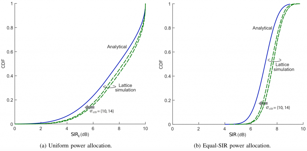
 and
and  . Figs. 2a-2b compare the simulations for
  dB with the analysis, and the agreement is now complete. The simulated average spectral efficiency with a uniform power allocation is
  b/s/Hz/user while (2) gives
  b/s/Hz/user.
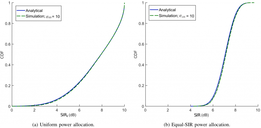
 –
– with very conservative premises) where these effects are rather minor, and the analysis is hence applicable.