All posts by Emil Björnson

The End of Independent Rayleigh Fading

When researchers study the basic properties of multi-antenna technologies, it is a common practice to model the channels using independent and identically distributed (i.i.d.) Rayleigh fading. This practice goes back many decades and is convenient since: 1) every antenna observes an independent realization of the channel; 2) each antenna is statistically equally good, so the ordering doesn’t matter; 3) the channel coefficients are complex Gaussian distributed, which leads to convenient mathematics.

The i.i.d. Rayleigh fading model has become the baseline that is considered unless the research is explicitly focused on a different model. When using the model to study spatial diversity, the diversity gain becomes proportional to the number of antennas. When characterizing the ergodic capacity of Massive MIMO, one can derive simple closed-form bounds where the SINR is proportional to the number of antennas. Both results are correct, but their generality is limited by the generality of the underlying fading model. Hence, it is important to know under what conditions i.i.d. Rayleigh fading can be observed.

When i.i.d. fading might occur

In isotropic scattering environments, where the multi-path components are uniformly distributed over all directions (in three dimensions), the fading realizations observed at two points have a correlation determined by the distance d between them. More precisely, the cross-correlation is sinc(2d/λ), where λ is the wavelength. The sinc function is zero when the argument is a non-zero integer, thus the fading realizations at two different points are uncorrelated if and only if they are separated by an integer multiple of λ/2. For example, d = λ/2, λ, 3λ/2, etc. Since the channel coefficients are Gaussian distributed in isotropic fading, uncorrelated fading results in independent fading.

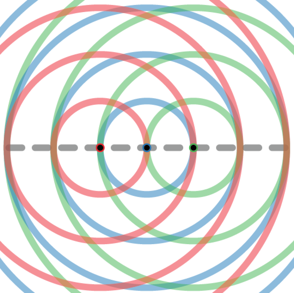
The figure above illustrates a setup where 3 antennas are deployed on the dashed line with a separation of λ/2. The red circles around the “red antenna” show at which locations one can observe fading realizations that are independent of the observation made at the red antenna. The circles have radius λ/2, λ, 3λ/2, etc. The blue and green circles have the same meanings for the blue and green antennas, respectively. Since all the antennas are deployed on the circles of the other antennas, they will observe mutually uncorrelated (independent) fading. This will give rise to i.i.d. Rayleigh fading.

Suppose we want to deploy a fourth antenna. To retain an i.i.d. fading distribution, we must put it at a point where a red, a blue, and a green circle intersect. As indicated by the figure, such points are only be found along the dashed line. Hence, a uniform linear array (ULA) with λ/2-separation between the adjacent antennas will observe i.i.d. fading if deployed in an isotropic scattering environment.

When i.i.d. fading cannot occur

Apart from the ULA example, there is essentially no other case where i.i.d. fading can occur. This is important since two-dimensional planar arrays are becoming standard, for example, when deploying Massive MIMO in cellular networks. Even if we allow ourselves to deviate from the isotropic scattering assumption, any physically accurate stochastic channel model for planar arrays exhibits correlation. This is proved in the paper “Spatially-Stationary Model for Holographic MIMO Small-Scale Fading“.

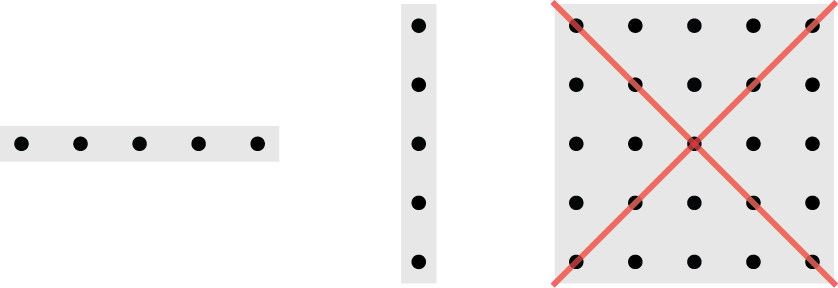
The horizontal and vertical ULAs in the figure above can observe i.i.d. fading, while the planar array cannot; even if the horizontal and vertical antenna spacing is λ/2, the spacings along the diagonals are different.

Looking further into the future, two new array concepts are currently receiving attention from the research community:

  1. Large intelligent surfaces (LIS);
  2. Reconfigurable intelligent surfaces (RIS).

LIS are large active arrays, while RIS are large passive arrays with elements that scatter incident signals in a semi-controllable fashion. In both cases, the word “surface” signifies that at a planar array, or even a three-dimensional array, is considered. Hence, these arrays can never observe i.i.d. fading—it is physically impossible. Moreover, a key characteristic of LIS and RIS is that the element spacing is smaller than λ/2 (to approximate a continuously controllable surface), which is yet another reason for obtaining spatial channel correlation. It is therefore worrying that several early papers on these topics are making use of the i.i.d. fading model: the analysis might be beautiful but the results are insignificant since they cannot be observed in practice.

The way forward

Even if we have reached the end of the road for the i.i.d. Rayleigh fading model, we don’t have to wander into the darkness. We just need to switch to utilizing the more general spatially correlated Rayleigh fading model. There is already a rich literature on how to design communication systems for such channels. My book “Massive MIMO networks” is one possible starting point, but not the only one.

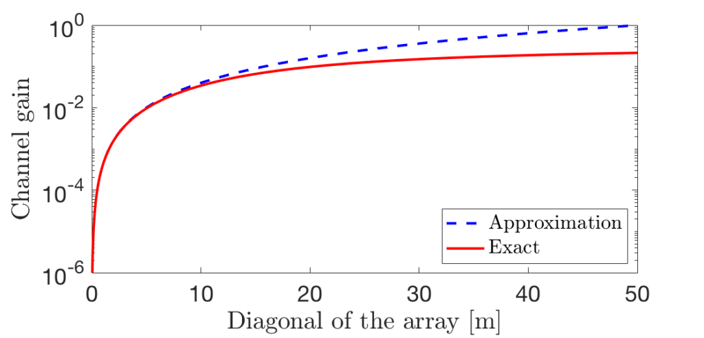
To make the transition to physically accurate models easier, I have co-authored the paper “Rayleigh Fading Modeling and Channel Hardening for Reconfigurable Intelligent Surfaces“, which derives a spatial correlation model for LIS and RIS in isotropic scattering environments. It can take the role as the new baseline channel model that is used when no other specific channel model is studied. We also elaborate on why the classical “Kronecker approximation” of spatial correlation matrices is inaccurate; for example, it results in i.i.d. fading also for planar arrays.

Reciprocity-based Massive MIMO in Action

I have written several posts about Massive MIMO field trials during this year. A question that I often get in the comment field is: Have the industry built “real” reciprocity-based Massive MIMO systems, similar to what is described in my textbook, or is something different under the hood? My answer used to be “I don’t know” since the press releases are not providing such technical details.

The 5G standard supports many different modes of operation. When it comes to spatially multiplexing of users in the downlink, the way to configure the multi-user beamforming is of critical importance to control the inter-user interference. There are two main ways of doing that.

The first option is to let the users transmit pilot signals in the uplink and exploit the reciprocity between uplink and downlink to identify good downlink beams. This is the preferred operation from a theoretical perspective; if the base station has 64 transceivers, a single uplink pilot is enough to estimate the entire 64-dimensional channel. In 5G, the pilot signals that can be used for this purpose are called Sounding Reference Signals (SRS). The base station uses the uplink pilots from multiple users to select the downlink beamforming. This is the option that resembles what the textbooks on Massive MIMO are describing as the canonical form of the technology.

The second option is to let the base station transmit a set of downlink signals using different beams. The user device then reports back some measurement values describing how good the different downlink beams were. In 5G, the corresponding downlink signals are called Channel State Information Reference Signal (CSI-RS). The base station uses the feedback to select the downlink beamforming. The drawback of this approach is that 64 downlink signals must be transmitted to explore all 64 dimensions, so one might have to neglect many dimensions to limit the signaling overhead. Moreover, the resolution of the feedback from the users is limited.

In practice, the CSI-RS operation might be easier to implement, but the lower resolution in the beamforming selection will increase the interference between the users and ultimately limit how many users and layers per user that can be spatially multiplexed to increase the throughput.

New field trial based on SRS

The Signal Research Group has carried out a new field trial in Plano, Texas. The unique thing is that they confirm that the SRS operation was used. They utilized hardware and software from Ericsson, Accuver Americas, Rohde & Schwarz, and Gemtek. A 100 MHz channel bandwidth in the 3.5 GHz band was considered, the downlink power was 120 W, and a peak throughput of 5.45 Gbps was achieved. 8 user devices received two layers each, thus, the equipment performed spatial multiplexing of 16 layers. The setup was a suburban outdoor cell with inter-cell interference and a one-kilometer range. The average throughput per device was around 650 Mbps and was not much affected when the number of users increased from one to eight, which demonstrates that the beamforming could effectively deal with the interference.

It is great to see that “real” reciprocity-based Massive MIMO provides such great performance in practice. In the report that describes the measurements, the Signal Research Group states that not all 5G devices support the SRS-based mode. They had to look for the right equipment to carry out the experiments. Moreover, they point out that:

Operators with mid-band 5G NR spectrum (2.5 GHz and higher) will start deploying MU-MIMO, based on CSI-RS, later this year to increase spectral efficiency as their networks become loaded. The SRS variant of MU-MIMO will follow in the next six to twelve months, depending on market requirements and vendor support.

The following video describes the measurements in further detail:

Active and Passive Antennas

If you are an academic physical-layer researcher, like me, you might be used to treating the base station as a single unit that takes a digital data signal as input and then outputs an electromagnetic radio wave (or the opposite in the uplink). The reality is quite different, or at least it used to be.

A traditional base station consists of three main components: a baseband unit (BBU) that takes care of digital signal processing, a radio unit that creates the analog radio-frequency (RF) signal, and a passive antenna that emits the RF signals with a constant radiation pattern. Due to the size and weight constraints of masts and towers, the radio and BBU are deployed underneath and there is a long RF feeder cable between the antenna and radio, resulting in substantial power losses. This is illustrated as “Step 1” in the figure below. A single BBU can support multiple radios that are deployed on the same site, which might cover different frequency bands or cell sectors (this is not illustrated).

Figure: The evolution of base station technology has gone through three main steps. In Step 1, the antenna is in the mast while the radio and BBU are underneath. The short blue cable sends digital baseband signals while the long purple cable sends analog RF signals. In Step 2, the radio is next to the antenna, so the purple RF cable is shorter. In Step 3, the antenna and radio are integrated into a single box. Multiple antennas and radios can be contained in the same box, which is called an AAS. The BBU can either be located underneath the AAS or “in the cloud”.

Now when the radio hardware has reduced in size, it is common to use remote radio units that are deployed in the tower, close to the antenna instead of close to the BBU. This is denoted as “Step 2” in the figure above and became common in the 4G era. Only a short RF feeder cable is then needed, while an optical fiber can be drawn from the BBU to the radio. The next step in the development is active antennas that integrate the antenna and radio into a single unit. There are many types of active antennas, from single-antenna units with constant radiation patterns to Massive MIMO antennas that adapt the radiation patterns by beamforming. To distinguish these things, the term advanced antenna system (AAS) is being used in the industry to refer to active Massive MIMO antenna arrays. This setup is denoted as “Step 3” in the figure and is becoming the dominating approach in the 5G era. To limit the capacity of the optical fiber between the AAS and BBU, an AAS might perform a limited set of baseband processing to compress/decompress the signals.

In summary, the latest radio-integrated active antennas are quite similar to what physical-layer researchers have been imaging for a while: A single unit that takes digital signals as input and emits an RF signal. Small cells can even include the BBU in the active antenna, while macro cell deployments purposely keep the BBU separate so it can be shared between multiple active antennas (it can even be moved to a nearby “cloud” computer). The advent of AAS technology is a key enabling factor for Massive MIMO deployment; a single box with 64 antennas and 64 radios can be made rather compact, while a deployment with 64 separate antenna boxes, 64 separate radio units, and an equal number of cables wouldn’t make practical sense.

Cross-Talk in MIMO Transmitters (In Memoriam of Professor Peter Händel)

I received an email in late August 2019 from my former boss at KTH, Professor Peter Händel. He had been working for many years on the modeling of hardware imperfections in wireless transceivers. Our research journeys had recently crossed since he had written several papers on the modeling of imperfections in MIMO transmitters and their impact on communication performance. I have been working on similar things but using far less sophisticated models.

The essence of the email was that he wanted us to write a paper together, but the circumstances came as a chock. Peter had been sick for a while and it turned out to be a terminal illness. He asked me to finalize a manuscript that he had initiated. I agreed and we exchanged a few emails but just as I and my postdoc were about to begin the editing of Peter’s manuscript, he passed away on September 15, 2019.

Impact of Backward Crosstalk in MIMO Transmitters

The manuscript considers a type of hardware impairment called backward crosstalk. It can be a major issue in the design of multi-antenna transmitters, but is generally overlooked by communication engineers. The issue arises when you build an antenna-integrated radio, for example, a Massive MIMO array with many antenna elements, power amplifiers, and radio-signal generators in a compact box. In this case, the output signal from one power amplifier will leak into the inputs of the neighboring power amplifiers. Even if the leakage is small in relative terms, it can still have a non-negligible impact since the output power of an amplifier is much higher than the input power. A small fraction of a large power value can still be rather large. In addition to this kind of backward crosstalk between amplifiers, there is also forward crosstalk in practice but it can be neglected for the very same reason.

This figure from the figure illustrates how the output signals r1, r2 from two neighboring power amplifiers are leaking into each other. The variables κ1, κ2 are representing the strength of this backward crosstalk.

We managed to finalize the manuscript, thanks to the excellent work by my postdoc Özlem Tuğfe Demir. The paper is now available:

Peter Händel, Özlem Tuğfe Demir, Emil Björnson, Daniel Rönnow, “Impact of Backward Crosstalk in 2×2 MIMO Transmitters on NMSE and Spectral Efficiency,” IEEE Transactions on Communications, vol. 68, no. 7, pp. 4277-4292, July 2020.

The paper considers a system model containing backward crosstalk, as well as, power amplifier non-linearities and transmitter noise. We characterize the performance both at the transmitter side (the normalized mean-squared error) and at the receiver side (the spectral efficiency). In turns out that optimization based on these two metrics can lead to very different transmission strategies; from a spectral efficiency perspective, one can transmit at higher power and accept a higher level of distortion since the desired signal power is also growing. In the paper, we also demonstrate how the precoding can be adapted to partially compensate for the crosstalk.

This paper is just a first step towards modeling real hardware imperfections that are normally ignored in academia or lumped together into a single additive term characterized by the error-vector magnitude. In the last emails I received from Peter, he expressed his view that there is a lot of open problems to solve at the interface between proper modeling of communication hardware and the design of signal processing schemes. I agree with him and encourage anyone who is looking for open problems on MIMO communications to have a closer look at his final papers on this topic:

(I wrote this blog post in memoriam of Professor Peter Händel, who would have become 58 years today.)

Even Higher Spectral Efficiency in Massive MIMO Trials

There are basically two approaches to achieve high data rates in 5G: One can make use of huge bandwidths in mmWave bands or use Massive MIMO to spatially multiplex many users in the conventional sub-6 GHz bands.

As I wrote back in June, I am more impressed by the latter approach since it is more spectrally efficient and requires more technically advanced signal processing. I was comparing the 4.7 Gbps that Nokia had demonstrated over an 840 MHz mmWave band with the 3.7 Gbps that Huawei had demonstrated over 100 MHz of the sub-6 GHz spectrum. The former example achieves a spectral efficiency of 5.6 bps/Hz while the latter achieves 37 bps/Hz.

T-Mobile and Ericsson recently described a new field trial with even more impressive results. They made use of 100 MHz in the 2.5 GHz band and achieved 5.6 Gbps, corresponding to a spectral efficiency of 56 bps/Hz; an order-of-magnitude more than one can expect in mmWave bands!

The press release describes that the high data rate was achieved using a 64-antenna base station, similar to the product that I described earlier. Eight smartphones were served by spatially multiplexing and each received two parallel data streams (so-called layers). Hence, each user device obtained around 700 Mbps. On average, each of the 16 layers had a spectral efficiency of 3.5 bps/Hz, thus 16-QAM was probably utilized in the transmission.

I think these numbers are representative of what 5G can deliver in good coverage conditions. Hopefully, Massive MIMO based 5G networks will soon be commercially available in your country as well.

What Happens When Arrays Become Physically Large?

Massive MIMO is all about using large arrays to transmit narrow beams, thereby increasing the received signal power and enabling spatial multiplexing of signals in different directions. Importantly, the words “large” and “massive” have relative meanings in this context: they refer to having many transceiver chains, which leads to many more spatial degrees of freedom in the beamforming design than in previous cellular technologies. However, the physical sizes of the 5G Massive MIMO arrays that are being deployed are similar to previous base station equipment. The reason is that the number of radiating elements is roughly the same and this is what determines the physical size.

What if we would deploy physically large arrays?

Since base station arrays are deployed at elevated places, many tens of meters from the users, 5G antenna arrays will look small from the viewpoint of the user. This situation might change in the future, when moving beyond 5G. Suppose we would cover the entire facade of a building with antennas, as illustrated in Figure 1, then the array would be physically large, not only feature a large number of transceiver chains.

Figure 1: A 5G Massive MIMO array has many antennas but is not physically large. This blog post considers physically large arrays that might be deployed over an entire building.

There are unusual wireless propagation phenomena that occur in such deployments and these have caught my attention in recent years. A lot of research papers on Massive MIMO consider the asymptotic regime where the number of antennas (transceiver chains) goes to infinity, but the channel models that are being used break down asymptotically. For example, the received signal power goes to infinity although the transmitted power is finite, which is physically impossible.

This inconsistency was a reason for why I didn’t jump onto the Massive MIMO train when it took off in 2010, but waited until I realized that Marzetta’s mind-blowing asymptotic results are also applicable in many practical situations. For example, if the users are at least ten meters away from the base station, we can make use of thousands of antennas before any inconsistencies arise. The asymptotic issues have been stuck in my mind ever since but now I have finally found the time and tools needed to characterize the true asymptotic behaviors.

Three important near-field characteristics

Three phenomena must be properly modeled when the user is close to a physically large array, which we call the array’s near-field. These phenomena are:

  1. The propagation distance varies between the different antennas in the array.
  2. The antennas are perceived to have different effective areas since they are observed from different angles.
  3. The signal losses due to polarisation mismatch vary due to the different angles.

Wireless propagation channels have, of course, always been determined by the propagation distances, effective antenna areas, and polarisation losses. However, one can normally make the approximation that they are equal for all antennas in the array. In our new paper “Power Scaling Laws and Near-Field Behaviors of Massive MIMO and Intelligent Reflecting Surfaces“, we show that all three conditions must be properly modeled to carry out an accurate asymptotic study. The new formulas that we present are confirming the intuition that the part of the array that is closest to the user is receiving more power than the parts that are further away. As the array grows infinitely large, the outer parts receive almost nothing and the results comply with fundamental physics, such as the law of conservation of energy.

You might have heard about the Fraunhofer distance, which is the wavelength-dependent limit between the near-field and far-field of a single antenna. This distance is not relevant in our context since we are not considering the radiative behaviors that occur close to an antenna, but the geometric properties of a large array. We are instead studying the array’s near-field, when the user perceives an electrically large array. The result is wavelength-independent and occurs approximately when the propagation distance is shorter than the widest dimension of the array. This is when one must take the three properties above into account to get accurate results. Note that it is not the absolute size of the array that matters but how large it is compared to the field-of-view of the user.

Figure 2 illustrates this property by showing the channel gain (i.e., the fraction of the transmitted power that is received) in a setup with an isotropic transmit antenna that is 10 m from the center of a square array. The diagonal of the array is shown on the horizontal axis. The solid red curve is computed using our new accurate formula, while the blue dashed curve is based on the conventional far-field approximation. The curves are overlapping until the diagonal is 10 m (same as the propagation distance). The difference increases rapidly when the array becomes larger (notice the logarithmic scale on the vertical axis). When the diagonal is 50 m, the approximation errors are extreme: the channel gain surpasses 1, which means that more power is received than was transmitted.

Figure 2: The channel gain when transmitting from a user that is 10 m from a square array. The conventional far-field approximation is accurate until the array becomes so large that one must take the three near-field characteristics into account.

There are practical applications

There are two ongoing lines of research where the new near-field results and insights are useful, both to consolidate the theoretical understanding and from a practical perspective.

One example is the physically large and dense Massive MIMO arrays which are being called large intelligent surfaces and holographic MIMO. These names are utilized to distinguish the analysis from the physically small Massive MIMO products that are now being deployed in 5G. Another example is the “passive” metasurface-based arrays that are being called reconfigurable intelligent surfaces and intelligent reflecting surfaces. These are arrays of scattering elements that can be configured to scatter an incoming signal from a transmitter towards a receiver.

We are taking a look at both of these areas in the aforementioned paper. In fact, the reason why we initiated the research last year is that we wanted to understand how to compare the asymptotic behaviors of the two technologies, which exhibit different power scaling laws in the far-field but converge to similar limits in the array’s near-field.

If you would like to learn more, I recommend you to read the paper and play around with the simulation code that you can find on GitHub.

Machine Learning for Massive MIMO Communications

Since the pandemic made it hard to travel over the world, several open online seminar series have appeared with focus on different research topics. The idea seems to be to give researchers a platform to attend talks by international experts and enable open discussions.

There is a “One World Signal Processing Seminar Series” series, which has partially considered topics on multi-antenna communications. I want to highlight one such seminar. Professor Wei Yu (University of Toronto) is talking about Machine Learning for Massive MIMO Communications. The video contains a 45 minute long presentation plus another 30 minutes where questions are being answered.

There are also several other seminars in the series. For example, I gave a talk myself on “A programmable wireless world with reconfigurable intelligent surfaces“. On August 24, Prof. David Gesbert will talk about “Learning to team play”.